
使用 R 进行离散事件模拟:医院容量规划。
4.97/5 (24投票s)
用于规划床位有限的肿瘤医院容量的模拟模型。R 脚本在 R Studio 上运行或通过 PHP 调用。

引言
繁忙的医疗机构由于患者流量的显著增加、与为这些患者提供护理相关的成本以及预算限制而不断面临挑战。为了帮助决策者最好地利用现有资源,将建模和模拟应用于医院运营,以评估当前策略的效率并预测未来可能应用于系统的任何变化的结果。
模型是数学框架,选择以足够的细节水平表示现实的某些方面,以促进对医疗保健决策后果的估计,并允许将复杂系统简化为其基本要素。模型被认为是健康技术评估中必不可少的工具。
系统模拟是模型的计算机操作,它使得在实际实施策略之前,可以研究系统属性、操作特性、评估不同的操作策略、得出结论并根据模拟结果做出行动决策。它是一个有用的工具,可以指导现有资源利用策略的改进,并协助基于数据收集和信息技术规划和设计新策略。
建模过程大致可分为两个不同的组成部分
1-问题的概念化
将医疗保健过程的知识转化为简化的问题表示
2-模型的概念化
指导选择满足所研究问题需求的建模技术。
此外,所研究问题的性质、目标人群、结果表示的时间范围以及项目目标对模型结构、填充所需数据、分析视角和模型报告具有重大影响。
医疗系统专家在问题概念化和模型规范开发中扮演着重要角色。问题的初步概念化应提供问题的完整图景,而不受数据可用性的限制。缺失或劣质数据对模型结构的影响应通过敏感性分析进行评估。
有许多决策分析模型可用。最基本的形式是使用决策树,它们是患者可能经历的所有可能情景以及每个情景在分支末尾的预期结果的图表。树分支模型所有可能的结果及其相关的概率。当结果集很小且时间范围短时,决策树效果很好。在建模癌症等慢性疾病时,参数不是随时间变化的,事件发生时间起着重要作用,事件也可能复发。在这些情况下,马尔可夫模型更受青睐。马尔可夫模型更好地处理长时间范围、事件发生时间以及复发事件。
马尔可夫模型是基于队列的模型,其中假设的同质患者队列通过定义的健康状态移动。时间以周期表示,在此期间患者可以 (a) 保持其当前的健康状态,(b) 移动到另一个健康状态,或 (c) 移动到终止状态(死亡),具有一定的转移概率。
在模拟过程中,可以积累不同策略的质量调整生命年 (QALY) 或成本等结果,然后进行比较。
尽管基于队列的模型相对简单,但在某些情况下必须表示个体层面的结果。此外,马尔可夫模型依赖于“马尔可夫假设”,即转移概率不依赖于历史,这使得马尔可夫模型“无记忆”。这可以通过增加状态数来解决。如果所需状态数变得太大,个体模拟是更好的替代方案。它还允许更好地表示特征的异质性。

实施个体层面模拟的一种方法是离散事件模拟 (DES),它是借鉴工程和运筹学方法的一种改编。DES 以定义的健康状态和可以发生在个体身上并使他们从一个状态转移到另一个状态的事件以及这些事件的后果来表示问题。
背景
在以下情况下,DES 是首选的模拟技术:
• 模型具有非常多的状态
• 模型中需要表示资源竞争和队列形成,以帮助缩短服务等待时间并回答资源分配问题。
• 需要在模型中表示个体之间的交互
离散事件模拟对系统进行建模,以比较不同的策略并确定最能利用所研究系统的策略。DES 的核心概念是实体、属性、事件、资源、队列和时间。实体是感兴趣的对象(通常是医疗保健模型中的患者),它们具有影响经历某些事件概率的属性。随着时间的推移,它们会竞争资源并进入队列。
事件可以是临床状况,例如癌症复发,或资源使用,例如床位利用,这些事件可以以任何逻辑顺序发生和复发。由患者竞争资源形成的队列可以通过各种服务纪律表示,例如“先进先出”或根据所研究系统中使用的纪律的“基于优先级”的纪律。
DES 的离散时间处理性质意味着模拟在事件发生的“离散”点上向前推进。模型推进到下一个事件,无需不必要的中间计算,这使得 DES 计算速度大大加快。
DES 建模过程的阶段
开发 DES 的第一步是定义所研究的系统以及可能在该系统中发生在个体身上的相关事件。这通过执行模型结构来辅助,其中识别所有可能的场景及其所需的参数。下一步是使用预收集的数据估计这些参数;如果所需数据不可用或质量差,可以咨询系统操作专家进行数据获取,并应验证他们的回答。如果专家获取的数据不具有适当的有效性,则模型应仅作为构建模型所需进一步数据收集的指南。
模型实施涉及将概念模型结构转换为计算机程序。可以使用 DES 专用软件填充和分析模型,该软件可以通过动画更好地可视化问题,并且非专家也易于应用。另一种方法是使用通用编程语言,例如“R”。

通用编程语言在表示系统细节方面更灵活,提供更短的模拟运行时间,并且更少依赖商业软件。然而,它们不提供花哨的动画,并且涉及为包函数编写更多代码(例如:用于制定事件列表、队列形成、资源利用和从概率分布中采样的代码),这使得其使用更复杂,并且需要大量的代码调试。
模型输出可能包括平均值或值分布。最佳实践建议,如果模型运行之间的输出值差异小于 5%(或根据设置阈值为 1%),则输出的稳定性被认为是可接受的。通过运行更多实体、增加时间范围或在模型中运行更多复制来提高稳定性,具体取决于所模拟系统的性质。
应应用验证技术以确保模型准确地代表现实。应进行敏感性分析以优化模拟模型并识别对模型具有显著影响的变量。
在 DES 报告中,应提供 DES 结构和逻辑的通用和详细表示,以及详细的事件文档图,因为它们对于建模者在展示模型方法和结果时至关重要。
使用代码
首先,您需要安装 R 和 R-studio(先安装 R,然后安装 R-studio)。我们使用“r-simmer”包来实现 DES,如下文所述。在本文中,我们使用了 r-simmer 版本 3.3。该包及其依赖项的完整安装文档在此处详细描述。本文随附的代码将在 R studio 中运行。另一个选项是按照本文中描述的 php 脚本调用说明进行操作,但 R 脚本需要稍作修改,这些修改也在下面的“启用通过 PHP 调用”部分中进行了说明。
假设您有一家医院,有 30 张住院病床,用于收治患有特定疾病的患者。让我们假设所有收治的患者都将通过由 4 个治疗阶段组成的标准方案进行治疗。在编写代码之前,我们首先绘制了包含实体竞争资源(在本例中为床位)的概率、到达间隔时间 (IAT)、分布和优先级的决策树。一个非常简化的示例如下图所示。实际上,它可能会变得更加复杂,包含嵌套分支和其他附加属性。

关于函数...
seize()
在我们的示例中,我们使用“床位”作为资源。seize() 函数将使实体(患者)占用一定数量的资源(在此示例中,一名患者占用一张床位:amount=1)。这里的优先级表示该实体在与其他实体竞争相同资源时将具有优先级排名。优先级 8 意味着该实体将优先于优先级为 7 或更低的实体,但不会优先于优先级为 9 或更高的实体。

timeout()
此函数将返回实体在给定状态下花费的时间量。因此,如果此函数与 seize() 一起使用,这意味着实体将占用资源,时间量由此函数返回。

在此示例中,timeout() 函数将从均值为 31.5 天、标准差为 2 天的正态分布中返回一个随机值。
以“人类可读”的形式编写嵌套函数
作者没有编写嵌套函数,而是使用了 R 中的 `%>%`(也称为:管道)运算符。例如,如果您有 3 个嵌套函数,您将有两种方式来编写这些函数:要么是“经典”的嵌套混淆形式,要么是易于理解的管道形式。
例如,如果您有以下三个函数...

我们不会像这样编写嵌套函数...

我们这样写...

代码已详细注释以进行澄清。如果您在代码实施过程中遇到任何挑战,请在下方留言,我们的团队将尽快回复。
## Thanks to R-Simmer authors Bart Smeets and Inaki Ucar for their support
## Full R Package documentation is available here (https://cran.r-project.cn/web/packages/simmer/)
## Start
cat("\014") ## clear console
file.remove("envs.txt") ## remove output file if exists
rm(list=ls()) ## Reset Environment
## Input Simulation parameters
nbeds<-30 ## number of beds
myrep<-5 ## number of repetitions
period<-730 ## run for two years (365 * 2 = 730)
myIAT<-3.65 ## Inter Arrival Time (in Days) ## our time = 3.65 for 200 patients/730 day
NumGenPt<- 0 ## number of Patients to come at the exact time, default=0 (n-1)
envs <- lapply(1:myrep, function(i) { #### lapply() to repeat myrep times
library(simmer)
env <- simmer("DiseaseX-env")
############### START Implementation of Decision Tree ###################
## add a new patient trajectory
newpatient <- create_trajectory("DiseaseX_patient_path") %>%
## the use of function1() %>% function2() %>% function3()
## is the same as using function3(function2(function1()))
## if you need to set an attribute use set_attribute() function
set_attribute("health_attribute", function() rnorm(1,70,3))%>%
branch(function() sample(c(1,2),size=1,replace=T,prob=c(0.90,0.10)), continue=c(T, T),
### begin treatment Phase1
create_trajectory("Treatment_Phase1") %>%
seize("bed", amount = 1, priority = 1) %>%
## for counting purpose, use dummy resource like the following
seize("Treatment_Phase1_in", amount = 1, priority = 1) %>%
## use the proper distribution that match real distribution
timeout(function() rnorm(1, 31, 2)) %>%
release("bed", 1)%>%
set_attribute("health_attribute", function() rnorm(1,50,3))%>%
######### Discharge after Phase 1 ########
## again dummy resource for counting purpose
seize("gohome_after_Phase1", amount = 1, priority = 99) %>%
timeout(function() sample(c(4,5,6),1)) %>%
release("gohome_after_Phase1", 1)%>%
######### Discharge after Phase 1 ########
#================ begin phase 2 of treatment
branch(function() sample(c(1,2),size=1,replace=T,prob=c(0.964,0.036)), continue=c(T, T),
create_trajectory("Treatment_Phase2") %>%
seize("bed", amount = 1, priority = 9) %>%
seize("Treatment_Phase2_in", amount = 1, priority = 9) %>%
## 28 day
timeout(function() rnorm(1, 28, 2)) %>%
release("bed", 1)%>%
######### Discharge after Phase 2 ########
seize("gohome_after_Phase2", amount = 1, priority = 99) %>%
timeout(function() sample(c(4,5,6),1)) %>%
release("gohome_after_Phase2", 1)%>%
######### END Discharge after Phase 2 ########
#=============== begin phase 3 of treatment
branch(function() sample(c(1,2),size=1,replace=T,prob=c(0.752,0.248)), continue=c(T, T),
create_trajectory("Treatment_Phase3") %>%
seize("bed", amount = 1, priority = 8) %>%
seize("Treatment_Phase3_in", amount = 1, priority = 8) %>%
## 25 day
timeout(function() rnorm(1, 25, 2)) %>%
release("bed", 1) %>%
######### Discharge after Phase 3 ########
seize("gohome_after_phase3", amount = 1, priority = 99) %>%
timeout(function() sample(c(4,5,6),1)) %>%
release("gohome_after_phase3", 1)%>%
######### END Discharge after Phase 3 ########
#=============== begin phase 4 of treatment
branch(function() sample(c(1,2),size=1,replace=T,prob=c(0.99,0.01)), continue=c(T, T),
create_trajectory("Treatment_Phase4") %>%
seize("bed", amount = 1, priority = 8) %>%
seize("Treatment_Phase4_in", amount = 1, priority = 8) %>%
## 31.5 day
timeout(function() rnorm(1, 31.5, 2)) %>%
release("bed", 1) %>%
######### Discharge after Phase 4 ########
seize("gohome_after_phase4", amount = 1, priority = 99) %>%
timeout(function() sample(c(4,5,6),1)) %>%
release("gohome_after_phase4", 1)%>%
######### END Discharge after Phase 4 ########
#=====Relapse
branch(function() sample(c(1,2),size=1,replace=T,prob=c(0.2,0.8)), continue=c(T, T),
create_trajectory("relapse") %>%
seize("bed", amount = 1, priority = 8) %>%
seize("relapse", amount = 1, priority = 8) %>%
## 40 day
timeout(function() rnorm(1, 40, 2)) %>%
release("bed", 1)
,
create_trajectory("relapse_out") %>%
seize("relapse_out", amount = 1, priority = 1)
)
#=====END Relapse
,
create_trajectory("Phase4_out") %>%
seize("Phase4_out", amount = 1, priority = 1)
)
#=============End Phase 4
,
create_trajectory("Phase3_out") %>%
seize("Phase3_out", amount = 1, priority = 1)
)
#===============End phase 3
,
create_trajectory("Phase2_out") %>%
seize("Phase2_out", amount = 1, priority = 1)
)
#=================End phase 2
,
create_trajectory("Phase1_out") %>%
set_attribute("health_attribute", function() rnorm(1,90,3))%>%
seize("phase1_out", amount = 1, priority = 1)
)
############### END Implementation of Decision Tree ###################
env %>%
## add true resource
add_resource("bed", nbeds) %>%
### Note: only resources with defined capacity can be
### plotted in "Resource Utilization"
## add resources for counting purpose
add_resource("Treatment_Phase1_in", Inf) %>%
add_resource("Treatment_Phase2_in", Inf) %>%
add_resource("Treatment_Phase3_in", Inf) %>%
add_resource("Treatment_Phase4_in", Inf) %>%
add_resource("relapse", Inf) %>%
add_resource("gohome_after_Phase1", Inf) %>%
add_resource("gohome_after_Phase2", Inf) %>%
add_resource("gohome_after_phase3", Inf) %>%
add_resource("gohome_after_phase4", Inf) %>%
add_resource("Phase4_out", Inf) %>%
add_resource("Phase3_out", Inf) %>%
add_resource("Phase2_out", Inf) %>%
add_resource("phase1_out", Inf) %>%
add_resource("relapse_out", Inf) %>%
## Add "Disease-X patient" generator, we assumed exp distribution (from real data)
add_generator("test_patient", newpatient, function() c(rexp(1, 1/myIAT), rep(0, NumGenPt)), mon=2)
env %>% run(until=period) ## run the simulation until reach time specified
})
########################## Recording Output ###########
out <- capture.output(envs)
### output the environment log
cat(paste(Sys.time(),"### Number of Bed =",nbeds,"### Number of Replica =",myrep,"### my IAT =",myIAT,"### Replicate Summary: \n"), out, file="envs.txt", sep="\n", append=TRUE)
### get monitored attributes as dataframe
attr<-envs %>% get_mon_attributes()
### get monitored resources as dataframe
resources<-envs %>% get_mon_resources()
n_resources<-resources[resources$resource == "bed",] ## filter only true resource "bed"
### get monitored arrivals per resource as dataframe
arrivals<-envs %>% get_mon_arrivals(per_resource=T)
## filter only true resource "bed" i.e. filter out dummy resources
n_arrivals<-arrivals[arrivals$resource == "bed",]
### calculate waiting time per visit and ALOS and add to n_arrivals dataframe
n_arrivals$waiting <- n_arrivals$end_time - n_arrivals$start_time - n_arrivals$activity_time
n_arrivals$ALOS<-n_arrivals$activity_time
## sum the total ALOS per patient
## the next line works accurately only if myrep=1
## reason for not being accurate with more than one replication is that
## some patients will be created in one run but not in the other causing a
## significant impact on the mean.
## Next version of this code will fix this issue, till then, the display of results
## from the next line is limited by an "if(myrep==1)"
ALOS_n<-aggregate(n_arrivals$ALOS, by=list(n_arrivals$name), FUN=sum)
ALOS_n$x<-ALOS_n$x/myrep ## divide by number of replications
### get monitored arrivals NOT per resource as dataframe
arrivals_no_resource<-get_mon_arrivals(envs)
arrivals_no_resource$ALOS<-arrivals_no_resource$activity_time
arrivals_no_resource$waiting<-arrivals_no_resource$end_time - arrivals_no_resource$start_time - arrivals_no_resource$activity_time
### save arrivals dataframe as csv with time stamp
filename_a<-paste0("arrival_",Sys.time(),".csv")
filename_a<-gsub(":", "_", filename_a)
write.csv(arrivals,filename_a)
### save attr dataframe as csv with time stamp
filename_attr<-paste0("attributes_",Sys.time(),".csv")
filename_attr<-gsub(":", "_", filename_attr)
write.csv(attr,filename_attr)
### save arrivals_no_resources dataframe as csv with time stamp
filename_an<-paste0("arrival_no_res_",Sys.time(),".csv")
filename_an<-gsub(":", "_", filename_an)
write.csv(arrivals_no_resource,filename_an)
### save resources dataframe as csv with time stamp
filename_r<-paste0("resources_",Sys.time(),".csv")
filename_r<-gsub(":", "_", filename_r)
write.csv(resources,filename_r)
################ Text mining of environment log ###############
r<-grep("\\brelapse\\b",out) ## get row containing number of relapses
n<-grep('n_generated',out) ## get row containing count of generated patients
q<-grep("\\bbed\\b",out) ## get row containing queue at end of period
# extract numeric values from rows
relapse<-out[r]
for (i in 1:myrep){
last<-regexpr('(Inf)', relapse[i])
relapse[i]= substr(relapse[i], (last-3), (last-2))
}
relapse<-as.numeric(relapse)
relapse
newpatients<-out[n]
for (i in 1:myrep){
last<-regexpr('}', newpatients[i])
newpatients[i]= substr(newpatients[i], (last-5), (last-2))
}
newpatients<-as.numeric(newpatients)
newpatients
queue<-out[q]
for (i in 1:myrep){
last<-regexpr('(Inf)', queue[i])
queue[i]= substr(queue[i], (last-4), (last-2))
}
queue<-as.numeric(queue)
queue ##this calculate que now i.e. at time <period>
mydata<-data.frame(newpatients,relapse,queue)
write.csv(mydata, "my_log_data.csv")
################ END Text mining of environment log ###############
############### Start Plotting #############
library(gridExtra)
library(grid)
library(ggplot2)
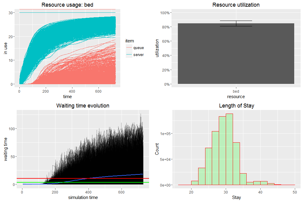
p1<-plot_resource_usage(envs, "bed", items = c("queue", "server"), steps = F)
p2<-plot_resource_utilization(envs, c("bed"))
p3<-plot_evolution_arrival_times(envs, type = "waiting_time")
p3<-p3 + geom_hline(yintercept=mean(arrivals_no_resource$waiting), colour="red", lwd=1)
p3<-p3 + geom_hline(yintercept=mean(n_arrivals$waiting), colour="green", lwd=1)
p4<-ggplot(data=n_arrivals, aes(n_arrivals$ALOS)) +
geom_histogram(aes(), breaks=seq(20, 50, by = 2), col="red", fill="green", alpha = .2) +
geom_density(col=2) +
labs(title="Length of Stay") +
labs(x="Stay", y="Count")
#cat("\014")
grid.arrange(p1, p2, p3,p4, ncol=2)
#########################################
# waiting time per resource = TRUE
summary(n_arrivals$waiting)
# waiting time per resource = FALSE
summary(arrivals_no_resource$waiting)
if(myrep==1){
# ALOS total visits per resource = TRUE
summary(ALOS_n$x)
}
# ALOS total visits per resource = FALSE
summary(arrivals_no_resource$ALOS)
# ALOS per visit (must be per resource = TRUE)
summary(n_arrivals$activity_time)
# Queue
summary(n_resources$queue)
# Patients generated
summary(mydata$newpatients)
更改变量 `myrep` 将通过 lapply() 运行多次模拟。
myrep<-10 ## 重复次数为 10 次

myrep<-100 ## 重复次数为 100 次

myrep<-1000 ## 重复次数为 1000 次
启用通过 PHP 调用
使用 PHP 调用 R 脚本非常简单。在本节中,我们将描述在 Windows 环境中使用 PHP 调用 R 脚本所需的几个步骤。第一步是创建包含本文随附的 R 脚本的 R 脚本文件 `MyModel.R`。需要注意的是,默认情况下,模型脚本输出的文件和图像保存到 R 的工作目录,这可能无法通过 Web 访问。因此,通过 Web 运行 R 脚本将需要对代码进行细微修改,以将输出保存到可访问的 Web 文件夹中。例如:
png(filename="c:/xampp/htdocs/model/output.png")
plot(MyDataPlot)
dev.off()
write.csv(MyData,"c:/xampp/htdocs/model/output.csv")
下一步是创建一个批处理文件 `MyTask.bat`,其中包含一行如下:
"C:\Rpath\R-3.2.3\bin\i386\Rscript.exe" MyModel.R
请记住将路径和 R 版本替换为您机器上的正确路径和版本。
我们最终需要从 PHP 文件中调用 `MyTask.bat`,但首先我们必须为 Windows 设置 XAMPP 服务器。让我们创建 `RunScript.php` 并将其放置在 Web 文件夹中。
<?php exec("MyTask.bat"); ?>
一旦我们通过 Web 浏览器访问 `RunScript.php` 页面,`MyTask.bat` 将被触发以运行 R 脚本 `MyModel.R`,并且输出(csv 文件、日志和图像)将保存到指定的 Web 文件夹中。
致谢
非常感谢 r-simmer 的作者 Bart Smeets 和 Iñaki Ucar 的支持。
完整的 R 包文档可在此处 获取。
参考文献
使用离散事件模拟建模:ISPOR-SMDM 建模良好研究实践工作组-4 的报告。