
使用 C# 绘制重复图
4.82/5 (11投票s)
一个绘制重复图并计算重复量化指标的应用程序。
引言
WinRQA 是一个使用 C# 编写的完整的 Windows 桌面应用程序,它可以绘制重现图并计算重现量化度量,以对时间序列进行重现量化分析(RQA)。

这个第一个版本只构建重现图并计算 RQA 度量,还允许对两个不同的图进行交叉或联合分析,但我计划将来继续扩展更多功能。
该应用程序是使用 Visual Studio 2013 创建的。
我添加了一些样本时间序列,有些来自 Lorenz、Henon 和 logistic 系统,一个带有白噪声,一个带有正弦信号,还有一个带有 EEG 数据,您可以使用它们来测试程序。
背景
重现分析并非易事,因此我必须假设您对此主题有所了解。无论如何,您可以 访问此网站,该网站致力于重现分析,您可以在其中找到信息和一些宝贵的资源。
您也可以 访问我的博客,其中我有一些与复杂时间序列分析主题相关的文章,也有西班牙语版本。
无论如何,我将尝试提供一个简短的摘要,说明重现分析是什么。
其思想是,如果我们有一个具有复杂结构的时间序列,它可能是具有多个独立变量的动态系统的一部分,并且可以包含允许近似重建完整系统相空间的信息。
将一维序列扩展到多维的程序是为每个额外维度创建一个新的时间序列,使用原始序列,但每个序列向前位移一个整数倍的恒定延迟。因此,第一维是原始序列,第二维是位移一个延迟的序列,第三维是位移两个延迟的序列,依此类推。
要构建重现图,我们首先创建一个平方数组,其中包含 n 维序列中每两个点之间的距离。每个 [i,j] 元素包含序列中第 i 个点和第 j 个点之间的距离。
然后,您可以简单地绘制距离数组,根据距离值给每个点着色,或者您可以决定一个最大距离(半径),低于该距离的两个距离被视为相等(即,两个点被视为重现)。
重现图显示了这些重现点,我们可以通过图中形成的点模式检测数据之间不易察觉的关系,或某些点序列动态的变化。
此外,还计算了一些量化度量,使用图中形成的对角线和垂直线的结构和分布,以及重现点的数量。这些度量有助于表征和分析正在研究的动态系统。
使用应用程序
在此版本的应用程序中,我们只能处理包含在文本文件中的时间序列,每行只有一个值,没有任何标题。
首先要做的是打开“文件”菜单并选择“打开...”选项。然后,通过对话框找到数据文件,重现图窗口将出现,最初是空的。

有两个工具栏,您可以在其中配置图的设置。在上方的工具栏中,设置 **延迟** 和 **嵌入** 维度以扩展时间序列,一个最大 **半径** 以考虑两个点是重现的(如果值为负数,则程序显示距离的彩色渐变),并选择一个 **范数** 来计算点之间的距离。
在下方的工具栏中,您可以定义用于构建图的时间序列窗口的 **开始** 和 **结束** 点,选择对角线(**线**)和垂直线(**VLine**)的最小长度,用于计算 **趋势** 度量的距离主对角线,并选择是否 **重缩放** 距离以标准化它们,除以最大或平均距离。
还有一些命令按钮。在上方的工具栏中,从左到右,有  按钮,用于绘制或重绘图,
 按钮,用于为重现点选择颜色,
 按钮用于将图显示为灰度或彩色比例,以防您为半径提供小于零的值。最后两个按钮是
  将重现图作为图像复制到剪贴板,以及
  将量化度量作为文本(制表符分隔)复制到剪贴板。
在下方的工具栏中, 按钮会显示一个帮助窗口,提供一个可视化界面,使用鼠标选择序列窗口的开始和结束点。
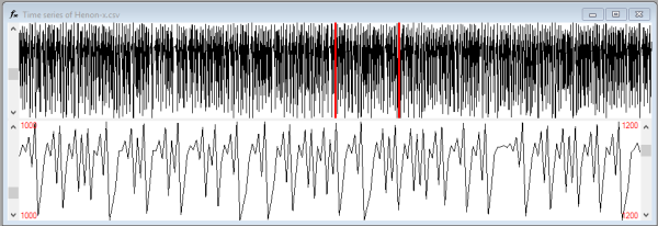
窗口的上半部分是完整的时间序列。您可以使用鼠标左键和右键单击来选择用于构建图的窗口的开始和结束点。通过序列左侧的滚动条,您可以在不改变窗口大小的情况下移动窗口。
下半部分是时间序列中选定的区间,通过其侧面的滚动条,您可以微调开始和结束点。这些设置会立即反映在重现图窗口的“开始”和“结束”文本框中。
该应用程序是 MDI(多文档界面)的,因此您可以同时打开多个时间序列。您可以拖动一个重现图并将其拖放到重现图窗口右侧的两个灰色面板之一上(两个图的大小和维度必须兼容)。
如果希望获得交叉重现图,请选择上方面板,其中距离是根据两个序列的点计算的(因此它们必须具有相同的嵌入维度)。
下方面板用于联合重现图,该图仅包含在两个重现图中相同位置重现的点。
理解代码
项目中的三个窗体是 **mainForm**(MDI 父窗体),**frmRecurrencePlot**(显示重现图和相关度量),以及 **frmTimeSeries**(用户可以在其中选择用于重现分析的时间序列窗口)。由于这些都是 WinForms 控件,我将不再深入介绍。
在 **Data** 命名空间中的四个类中,**NamedItem** 只是一个帮助程序,用于在下拉列表中以友好名称显示项,**VectorExport** 是另一个帮助类,用于在窗体之间拖放图,**DataFileManager** 封装了读取数据文件的逻辑,数据文件是每行包含一个时间序列值的文本文件。
所以,让我们详细检查最后一个类 **RecurrencePlot**,它实现了重现图本身。首先,有三个枚举用于配置图。
// Different kinds of distance between vectors
public enum Norm
{
      Euclidean, Minimum, Maximum
}
// Normalization applied to the distance matrix
public enum Rescaling
{
      None, Mean, Max
}
// Type of recurrence plot
public enum PlotType
{
      Normal, Cross, Joint
}
由于图显示的是向量之间的距离,因此 **Norm** 枚举指示我们使用哪种范数来计算它。欧几里得范数是向量分量平方差之和的平方根。最大范数是向量分量距离中的最大值,最小范数是最小值。
**Rescaling** 用于标准化距离,主要在需要交叉两个图时使用,它包括将每个距离除以最大距离或平均距离。
**PlotType** 指示应该构建哪种类型的重现图,Normal(绘制时间序列与自身重现),或 Cross / Joint(绘制两个不同时间序列或同一时间序列的两个部分之间的交叉/联合重现图)。
类变量如下:
// Plot parameters
private DataFileManager _data = null;
private float _radius = 0f;
private int _delay = 1;
private int _embed = 3;
private int _line = 2;
private int _vline = 2;
private int _trendK = 10;
private int _start = 0;
private int _end = 0;
private Norm _norm = Norm.Euclidean;
private Rescaling _rescaling = Rescaling.None;
private PlotType _type = PlotType.Normal;
// Internal measures
private float _maxDistance = 0f;
private float _meanDistance = 0f;
// Joint plot versions
private float _maxJDistance = 0f;
private float _meanJDistance = 0f;
// Vectors
private float[,] _vectors = null;
private float[,] _ovectors = null;
// Distance Matrix
private float[,] _dMatrix = null;
// Recurrence Matrix
private int[,] _rMatrix = null;
// Radius for Joint plot
private float _jRadius = 0f;
**_data** 是一个 DataFileManager,用于读取时间序列数据,**_radius** 是被视为重现的向量之间的最大距离,**_delay** 是用于将时间序列扩展到多维的延迟,**_embed** 是嵌入维度,**_line** 是最小对角线长度,**_vline** 是最小垂直线长度,**_trendK** 是用于计算 TREND RQA 度量的常数,它是此计算中要考虑的主对角线距离,**_start** 和 **_end** 是用于构建图的时间序列窗口的开始和结束点,**_norm** 包含使用的距离类型,**_rescaling** 用于标准化距离,**_type** 是要构建的重现图的类型,**_maxDistance** 是整个图中的最大距离,**_meanDistance** 是所有距离的平均值,**_maxJDistance** 和 **_meanJDistance** 对于联合重现图版本相同,**_vectors** 是用嵌入维度和延迟构建的向量,**_ovectors** 是另一个重现图的向量,用于交叉或联合,**_dMatrix** 是距离矩阵,**_rMatrix** 是重现矩阵,其中包含重现点的 0,或非重现点的非零值,最后,**_jRadius** 是在构建联合重现图时用于计算另一个图的向量之间距离的半径。
RQA 度量作为属性公开。
public float RR { get; private set; }
public float DET { get; private set; }
public float RATIO { get; private set; }
public float L { get; private set; }
public int LMAX { get; private set; }
public float DIV { get; private set; }
public float ENTR2 { get; private set; }
public float ENTRe { get; private set; }
public float TREND { get; private set; }
public float LAM { get; private set; }
public int VMAX { get; private set; }
public float TT { get; private set; }
有关这些度量的解释,您可以访问以下页面:http://www.recurrence-plot.tk/rqa.php。
几乎所有的全局变量都作为属性公开。由于对可接受的值组合存在一些限制,因此有一个辅助函数可以一次性为所有变量赋值。
public void SetAllValues(float radius,
    int delay,
    int embed,
    int line,
    int vline,
    int trendk,
    int start,
    int end,
    Norm norm,
    Rescaling
    rescaling,
    PlotType type)
布尔属性 **ColorScheme** 用于设置颜色(彩色或灰度)图例,以便在未定义用于将两个点视为重现的最小半径且图被绘制为距离渐变图时进行绘制。使用此函数,您可以将重现矩阵中的距离转换为颜色。
public Color GetPointColor(int level)
该类的核心是 **Process** 函数,它执行所有计算来构建重现图。首先要做的就是加载数据并使用提供的嵌入维度和延迟来构建向量数组。
_vectors = new float[Range, _embed];
_data.Open();
try
{
    _data.Seek(_start);
    int pos = 0;
    float[] values = new float[1000];
    int vlength = _data.ReadBuffer(values);
    while (pos < Range + (_delay * _embed - 1))
    {
        int ix = 0;
        while (ix < vlength)
        {
            // Reuse the value in all needed places, to avoid reprocess of the data
            for (int d = 0; d < _embed; d++)
            {
                int pd = (ix + pos) - (d * _delay);
                if (pd >= 0)
                {
                    if (pd / Range == 0)
                    {
                        _vectors[pd % Range, d] = values[ix];
                    }
                }
                else
                {
                    break;
                }
            }
            ix++;
        }
        // The data is read in chunks
        pos += values.Length;
        if (pos < Range + (_delay * _embed - 1))
        {
            vlength = _data.ReadBuffer(values);
        }
    }
}
finally
{
    _data.Close();
}
数据以 1000 个样本的块读取。向量都具有等于嵌入维度的坐标数,每个坐标包含时间序列在当前位置的值加上等于延迟乘以坐标索引的偏移量(ix, ix + delay, ix + 2*delay 等)。
这意味着相同的值可以成为一个以上向量的一部分。为了避免每个维度读取一次数据,内部循环将值放置在所有需要的地方。
下一步是构建这些向量之间的距离矩阵。矩阵中的每个位置 i,j 包含第 i 个向量和第 j 个向量之间的距离,因此,对于正常和联合图,矩阵相对于主对角线(称为身份线 LOI)是对称的,并且该对角线上的所有距离始终为 0,因为它们是每个向量与自身之间的距离。对于交叉重现图,第 i 个点和第 j 个点之间的距离与第 j 个点和第 i 个点之间的距离不相同,因此在这种情况下,我们必须处理整个矩阵。
// Now build and construct the distance matrix
_dMatrix = new float[Range, Range];
_meanDistance = 0f;
_maxDistance = 0f;
// Needed for Joint plot
float[,] jMatrix = null;
if (_type == PlotType.Joint)
{
    jMatrix = new float[Range, Range];
    _meanJDistance = 0f;
    _maxJDistance = 0f;
}
int ixc = 0;
int iyc = 0;
int maxdim = TypeofPlot == PlotType.Joint ? Math.Max(_embed, _ovectors.GetLength(1)) : _embed;
float _dcount = 0f;
if (TypeofPlot == PlotType.Cross)
{
    for (iyc = 0; iyc < Range; iyc++)
    {
        for (ixc = 0; ixc < Range; ixc++)
        {
            float sdif = InitialDistance;
            // Calculate distance
            for (int cv = 0; cv < maxdim; cv++)
            {
                sdif = Distance(_vectors[iyc, cv], _ovectors[ixc, cv], sdif);
            }
            //Store results in the matrixes
            if (_norm == Norm.Euclidean)
            {
                sdif = (float)Math.Sqrt(sdif);
            }
            _dcount++;
            _dMatrix[ixc, iyc] = sdif;
            _maxDistance = Math.Max(_maxDistance, sdif);
            _meanDistance += sdif;
        }
    }
}
else
{
    for (iyc = 0; iyc < Range; iyc++)
    {
        _dMatrix[iyc, iyc] = 0f;
        for (ixc = iyc + 1; ixc < Range; ixc++)
        {
            float sdif = InitialDistance;
            float jdif = InitialDistance;
            // Calculate distance
            for (int cv = 0; cv < maxdim; cv++)
            {
                switch (TypeofPlot)
                {
                    case PlotType.Normal:
                        sdif = Distance(_vectors[iyc, cv], _vectors[ixc, cv], sdif);
                        break;
                    case PlotType.Joint:
                        if (cv < _embed)
                        {
                            sdif = Distance(_vectors[iyc, cv], _vectors[ixc, cv], sdif);
                        }
                        if (cv < _ovectors.GetLength(1))
                        {
                            jdif = Distance(_ovectors[iyc, cv], _ovectors[ixc, cv], jdif);
                        }
                        break;
                }
            }
            //Store results in the matrixes
            if (_norm == Norm.Euclidean)
            {
                sdif = (float)Math.Sqrt(sdif);
            }
            _dcount++;
            _dMatrix[ixc, iyc] = sdif;
            _dMatrix[iyc, ixc] = sdif;
            _maxDistance = Math.Max(_maxDistance, sdif);
            _meanDistance += sdif;
            if (TypeofPlot == PlotType.Joint)
            {
                if (_norm == Norm.Euclidean)
                {
                    jdif = (float)Math.Sqrt(jdif);
                }
                jMatrix[ixc, iyc] = jdif;
                jMatrix[iyc, ixc] = jdif;
                _maxJDistance = Math.Max(_maxJDistance, jdif);
                _meanJDistance += jdif;
            }
        }
    }
}
_meanDistance /= _dcount;
_meanJDistance /= _dcount;
根据我们正在构建的重现图的类型,计算距离的方式会有所不同。在普通图中,会计算向量之间的距离,但在交叉重现图的情况下,我们有两个不同的向量集,并且距离是在一个集合的第 i 个向量和另一个集合的第 j 个向量之间计算的。
在联合重现图的情况下,我们也有两个向量集,但我们构建了两个独立的距离矩阵,一个用于每个向量集。
除了矩阵之外,还会计算距离的最大值和平均值。
下一步是根据需要进行重缩放,除以最大距离,将所有距离保留在 0 到 1 之间,或除以平均距离。
// Rescaling if needed
switch (_rescaling)
{
    case Rescaling.Max:
        for (int x = 0; x < Range; x++)
        {
            for (int y = 0; y < Range; y++)
            {
                _dMatrix[x, y] /= _maxDistance;
                if (jMatrix != null)
                {
                    jMatrix[x, y] /= _maxJDistance;
                }
            }
        }
        _meanDistance /= _maxDistance;
        _maxDistance = 1f;
        break;
    case Rescaling.Mean:
        for (int x = 0; x < Range; x++)
        {
            for (int y = 0; y < Range; y++)
            {
                _dMatrix[x, y] /= _meanDistance;
                if (jMatrix != null)
                {
                    jMatrix[x, y] /= _meanJDistance;
                }
            }
        }
        _maxDistance /= _meanDistance;
        _meanDistance = 1f;
        break;
}
接下来,构建重现矩阵。重现点的计数存储在 **prec** 变量中,因为稍后将使用它来计算量化度量。如果距离小于半径,则两个点被视为重现。如果提供的半径小于 0,则矩阵存储与距离成比例的值以选择颜色或灰度,但如果它大于零,则矩阵包含重现点的 0 和非重现点的 255。同样,对于交叉重现图,过程略有不同。
// Build recurrence matrix
_rMatrix = new int[Range, Range];
// Count of recurrent points
int prec = 0;
// Number of points in the plot, excluding the diagonal and taking into account only a half of the matrix or all for the cross recurrence plot
int tpnt = TypeofPlot == PlotType.Cross ? Range * Range : (Range * (Range - 1)) / 2;
// Find recurrences
if (TypeofPlot == PlotType.Cross)
{
    for (iyc = 0; iyc < Range; iyc++)
    {
        for (ixc = 0; ixc < Range; ixc++)
        {
            // If radius is 0, the distances are scaled from 0 to 255, in order to create a gray scale
            // If radius > 0, then 0 is a recurrence, and 255 a not recurrent point
            int level = _radius < 0f ? (int)((_dMatrix[ixc, iyc] * ColorRange) / _maxDistance) : (_dMatrix[ixc, iyc] <= _radius ? 0 : 255);
            _rMatrix[ixc, iyc] = level;
            if (level == 0)
            {
                prec++;
            }
        }
    }
}
else
{
    for (iyc = 0; iyc < Range; iyc++)
    {
        for (ixc = iyc; ixc < Range; ixc++)
        {
            // If radius is 0, the distances are scaled from 0 to 255, in order to create a gray scale
            // If radius > 0, then 0 is a recurrence, and 255 a not recurrent point
            int level = _radius < 0f ? (int)((_dMatrix[ixc, iyc] * ColorRange) / _maxDistance) : (_dMatrix[ixc, iyc] <= _radius ? 0 : 255);
            if ((_radius >= 0) && (TypeofPlot == PlotType.Joint))
            {
                int level2 = jMatrix[ixc, iyc] <= _jRadius ? 0 : 255;
                if (level != level2)
                {
                    level = 255;
                }
            }
            _rMatrix[ixc, iyc] = level;
            if ((ixc != iyc) && (level == 0))
            {
                prec++;
            }
        }
    }
}
现在是时候计算重现量化度量了。这些是相关的变量。
// Histogram of diagonal line length
int[] pl = new int[Range - _line];
// Histogram of vertical line length
int[] pv = new int[Range - _vline];
// Count of points in every diagonal
float[] rr = new float[Range - 1];
// Sum of diagonal lengths
int spl = 0;
// Number of diagonal lines
int npl = 0;
// Sum of vertical lengths
int spv = 0;
// Number of vertical lines
int npv = 0;
// Max diagonal line length
int lmax = 0;
// Max vertical line length
int vlmax = 0;
// Entropy (log base 2)
double sppl = 0;
// Entropy (Natural log)
double spple = 0;
// Average diagonal line length
float avgl = 0f;
// Average vertical line length
float avgv = 0f;
// Average points in diagonals
float avgr = 0f;
// Trend
float tr = 0f
首先,长度大于或等于 **_line** 和 **_vline** 中提供值的对角线和垂直线被计数到变量 **npl** 和 **npv** 中,并且每条线的计数存储在直方图 **pl** 和 **pv** 中。对于正常图和联合图,只使用矩阵的一半,因为它是相对于主对角线对称的。主对角线不被计算在内。**rr** 变量存储每条对角线上的重现点的百分比,并用于计算趋势度量。如果我们正在构建交叉重现图,则必须处理整个重现矩阵。
if (TypeofPlot == PlotType.Cross)
{
    for (int l = 1; l < Range; l++)
    {
        int cl1 = 0;
        int cl2 = 0;
        for (int i = 0; i <= l; i++)
        {
            // Diagonal line length (Upper half of the matrix)
            if (_rMatrix[i, i + ((Range - 1) - l)] == 0f)
            {
                cl1++;
            }
            else
            {
                if (cl1 >= _line)
                {
                    pl[cl1 - _line]++;
                    npl++;
                }
                cl1 = 0;
            }
            // Diagonal line length (Lower half of the matrix)
            if (l < Range - 1) // Count only once the main diagonal
            {
                if (_rMatrix[i + ((Range - 1) - l), i] == 0f)
                {
                    cl2++;
                }
                else
                {
                    if (cl2 >= _line)
                    {
                        pl[cl2 - _line]++;
                        npl++;
                    }
                    cl2 = 0;
                }
            }
        }
        if (cl1 >= _line)
        {
            pl[cl1 - _line]++;
            npl++;
        }
        if (cl2 >= _line)
        {
            pl[cl2 - _line]++;
            npl++;
        }
    }
    for (int l = 0; l < Range; l++)
    {
        int cv = 0;
        for (int i = 0; i < Range; i++)
        {
            // Vertical line length
            if (_rMatrix[l, i] == 0f)
            {
                cv++;
            }
            else
            {
                if (cv >= _vline)
                {
                    pv[cv - _vline]++;
                    npv++;
                }
                cv = 0;
            }
        }
        if (cv >= _vline)
        {
            pv[cv - _vline]++;
            npv++;
        }
    }
}
else
{
    for (int l = 0; l < Range - 1; l++)
    {
        int cl = 0;
        int cv = 0;
        float cr = 0f;
        for (int i = 0; i <= l; i++)
        {
            // Diagonal line length
            if (_rMatrix[(Range - 1) - i, l - i] == 0f)
            {
                cl++;
                cr += 1f;
            }
            else
            {
                if (cl >= _line)
                {
                    pl[cl - _line]++;
                    npl++;
                }
                cl = 0;
            }
            // Vertical line length
            if (_rMatrix[l + 1, i] == 0f)
            {
                cv++;
            }
            else
            {
                if (cv >= _vline)
                {
                    pv[cv - _vline]++;
                    npv++;
                }
                cv = 0;
            }
        }
        rr[l] = cr / (float)(l + 1);
        if (cl >= _line)
        {
            pl[cl - _line]++;
            npl++;
        }
        if (cv >= _vline)
        {
            pv[cv - _vline]++;
            npv++;
        }
    }
}
利用这些直方图,我们可以计算其他度量,如平均和最大对角线和垂直线长度、香农信息熵以及对角线分布相对于主对角线的趋势。TREND 度量不适用于交叉重现图。
// Calculate Max & Avg diagonal length, anmd entropy
for (int ip = 0; ip < pl.Length; ip++)
{
    spl += (ip + _line) * pl[ip];
    if (pl[ip] > 0)
    {
        avgl += (float)(ip + _line) * pl[ip];
        double p = (double)pl[ip] / (double)npl;
        sppl += p * Math.Log(p, 2);
        spple += p * Math.Log(p);
    }
    if (pl[ip] > 0)
    {
        lmax = ip + _line;
    }
}
// Calculate Max & Avg vertical line length
for (int ip = 0; ip < pv.Length; ip++)
{
    spv += (ip + _vline) * pv[ip];
    if (pv[ip] > 0)
    {
        avgv += (float)(ip + _vline) * pv[ip];
    }
    if (pv[ip] > 0)
    {
        vlmax = ip + _vline;
    }
}
// Finish the average and entropy calculations
sppl = -sppl;
spple = -spple;
if (npl != 0)
{
    avgl /= (float)npl;
}
if (npv != 0)
{
    avgv /= (float)npv;
}
for (int ir = rr.Length - _trendK; ir < rr.Length; ir++)
{
    avgr += rr[ir];
}
// Only calculate TREND to Normal and Joint recurrence plots
if (TypeofPlot != PlotType.Cross)
{
    for (int ir = rr.Length - _trendK; ir < rr.Length; ir++)
    {
        avgr += rr[ir];
    }
    // Terminate the trend calculation
    avgr /= (float)_trendK;
    float i2 = 0f;
    float n2 = (float)_trendK / 2f;
    for (int i = 0; i < _trendK; i++)
    {
        tr += ((float)(i + 1) - n2) * (rr[i] - avgr);
        i2 += ((float)(i + 1) - n2) * ((float)(i + 1) - n2);
    }
    tr *= 1000f;
    tr /= i2;
}
最后,计算完成并存储在相应的属性中。
// Store the values in the RQA properties
RR = (float)prec / (float)tpnt;
DET = (float)spl / (float)prec;
RATIO = (float)(spl * tpnt) / (float)(prec * prec);
L = avgl;
LMAX = lmax;
DIV = lmax > 0? 1f / (float)lmax: float.NaN;
ENTR2 = (float)sppl;
ENTRe = (float)spple;
TREND = tr;
LAM = (float)spv / (float)prec;
VMAX = vlmax;
TT = avgv;
绘图操作在一个单独的函数中完成,因此您可以在无需重新计算所有距离和度量的情况下重绘它。
public Bitmap DrawRecurrencePlot(int maxwidth, int maxheight, Color color)
关于此函数的唯一要说明的是,它会生成一个方形位图,重现矩阵中的每个位置至少有一个像素的最小边长。如果宽度和高度参数(通常是您希望绘制位图的窗口大小)允许每个位置使用多个像素,则位图将被缩放到最大可能大小。颜色参数用于绘制半径大于或等于零的图,这些图使用两种颜色绘制(背景始终为白色)。
int scale = Math.Max(1, Math.Min(maxwidth, maxheight) / Range);
Bitmap bmprp = new Bitmap(scale * Range, scale * Range);
目前就到这里。我的计划是将来添加一些图形工具来帮助确定图的参数,例如延迟、嵌入维度和半径,以及一些图,显示一些 RQA 度量的演变,因为一些图设置会发生变化。
感谢阅读!!!