
支持向量机 (SVM) 和简化 SMO 算法介绍
3.00/5 (6投票s)
SVM 和简化 SMO 算法介绍
引言
在机器学习中,支持向量机(SVM)是监督学习模型,其学习算法用于分析用于分类和回归分析的数据(维基百科)。本文是我学习的总结,主要参考文献可在参考文献部分找到。
支持向量机和序列最小优化(SMO)可在 [1]、[2] 和 [3] 中找到。SMO 简化版的详细信息及其伪代码可在 [4] 中找到。您还可以在 [5] 中找到 SMO 算法的 Python 代码,但对于刚开始学习机器学习的初学者来说,它很难理解。[6] 是为想要基本了解支持向量机的初学者准备的特别礼物。在本文中,我将基于 [4] 使用 Python 代码介绍 SVM 和 SMO 的简化版。
背景
在本文中,我们将考虑一个二元分类问题的线性分类器,标签为 y (y ϵ [-1,1]),特征为 x。SVM 将计算一个形式为

使用 f(x),我们可以预测 y = 1 if f(x) ≥ 0 and y = -1 if f(x) < 0。通过求解对偶问题(参考文献部分的公式 12, 13 [1]),f(x) 可以表示为
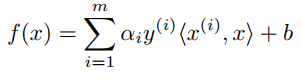
其中 αi (alpha i) 是解的拉格朗日乘子,<x(i),x> 称为 x(i) 和 x 的内积。f(x) 的 Python 版本可能看起来像这样
fXi = float(multiply(alphas,Y).T*(X*X[i,:].T)) + b
简化版 SMO 算法
简化版 SMO 算法接收两个 α 参数,αi 和 αj,并对它们进行优化。为此,我们遍历所有 αi,i = 1, . . . m。如果 αi 在某个数值容差范围内不满足 **Karush-Kuhn-Tucker 条件**,我们就从剩余的 m - 1 个 α 中随机选择一个 αj 并优化 αi 和 αj。以下函数将帮助我们随机选择 j
def selectJrandomly(i,m):
      j=i
      while (j==i):
            j = int(random.uniform(0,m))
      return j
如果在遍历所有 αi 的几次迭代后没有任何 α 被改变,则算法终止。我们还必须找到界限 L 和 H
- If y(i) != y(j), L = max(0, αj − αi), H = min(C, C + αj − αi)
- If y(i) = y(j), L = max(0, αi + αj − C), H = min(C, αi + αj)
其中 C 是正则化参数。上述内容的 Python 代码如下
if (Y[i] != Y[j]):
      L = max(0, alphas[j] - alphas[i])
      H = min(C, C + alphas[j] - alphas[i])
else:
      L = max(0, alphas[j] + alphas[i] - C)
      H = min(C, alphas[j] + alphas[i])
现在,我们将找到 αj 的值,该值由下式给出

Python 代码
alphas[j] -= Y[j]*(Ei - Ej)/eta
其中

Python 代码
Ek = fXk - float(Y[k])
eta = 2.0 * X[i,:]*X[j,:].T - X[i,:]*X[i,:].T - X[j,:]*X[j,:].T
如果此值超出界限 L 和 H,我们必须将 αj 的值裁剪到此范围内

以下函数将帮助我们裁剪 αj 的值
def clipAlphaJ(aj,H,L):
      if aj > H:
            aj = H
      if L > aj:
            aj = L
      return aj
最后,我们可以找到 αi 的值。该值由下式给出

其中 α(old)j 是优化前的 αj 值。Python 代码的一个版本可能看起来像这样
alphas[i] += Y[j]*Y[i]*(alphaJold - alphas[j])
优化 αi 和 αj 后,我们选择阈值 b

其中 b1

和 b2

b1 和 b2 的 Python 代码:
b1 = b - Ei- Y[i]*(alphas[i]-alphaIold)*X[i,:]*X[i,:].T - Y[j]*(alphas[j]-alphaJold)*X[i,:]*X[j,:].T
b2 = b - Ej- Y[i]*(alphas[i]-alphaIold)*X[i,:]*X[j,:].T - Y[j]*(alphas[j]-alphaJold)*X[j,:]*X[j,:].T
计算 W
优化 αi 和 αj 后,我们还可以计算 w,该值由下式给出

以下函数帮助我们从 αi 和 αj 计算 w
def computeW(alphas, dataX, classY):
      X = mat(dataX)
      Y = mat(classY).T
      m,n = shape(X)
      w = zeros((n,1))
      for i in range(m):
            w += multiply(alphas[i]*Y[i],X[i,:].T)
      return w
预测类别
我们可以根据 w 和 b 预测一个点属于哪个类别
def predictedClass(point, w, b):
      p = mat(point)
      f = p*w + b
      if f > 0:
            print(point," is belong to Class 1")
      else:
            print(point," is belong to Class -1")
简化版 SMO 算法的 Python 函数
现在,我们可以根据 [4] 中的伪代码创建一个用于简化版 SMO 算法的函数(命名为 simplifiedSMO)
输入
- C:正则化参数
- tol:数值容差
- max passes:在不改变的情况下遍历 α 的最大次数
- (x(1), y(1)), . . . , (x(m), y(m)):训练数据
输出
α:解的拉格朗日乘子
b:解的阈值
def simplifiedSMO(dataX, classY, C, tol, max_passes):
       X = mat(dataX);
       Y = mat(classY).T
       m,n = shape(X)
       # Initialize b: threshold for solution
       b = 0;
       # Initialize alphas: lagrange multipliers for solution
       alphas = mat(zeros((m,1)))
       passes = 0
       while (passes < max_passes):
              num_changed_alphas = 0
              for i in range(m):
                     # Calculate Ei = f(xi) - yi
                     fXi = float(multiply(alphas,Y).T*(X*X[i,:].T)) + b
                     Ei = fXi - float(Y[i])
                     if ((Y[i]*Ei < -tol) and (alphas[i] < C)) or ((Y[i]*Ei > tol)
                                  and (alphas[i] > 0)):
                           # select j # i randomly
                           j = selectJrandom(i,m)
                           # Calculate Ej = f(xj) - yj
                           fXj = float(multiply(alphas,Y).T*(X*X[j,:].T)) + b
                           Ej = fXj - float(Y[j])
                           # save old alphas's
                           alphaIold = alphas[i].copy();
                           alphaJold = alphas[j].copy();
                           # compute L and H
                           if (Y[i] != Y[j]):
                                  L = max(0, alphas[j] - alphas[i])
                                  H = min(C, C + alphas[j] - alphas[i])
                           else:
                                  L = max(0, alphas[j] + alphas[i] - C)
                                  H = min(C, alphas[j] + alphas[i])
                           # if L = H the continue to next i
                           if L==H:
                                  continue
                           # compute eta
                           eta = 2.0 * X[i,:]*X[j,:].T - X[i,:]*X[i,:].T - X[j,:]*X[j,:].T
                           # if eta >= 0 then continue to next i
                           if eta >= 0:
                                  continue
                           # compute new value for alphas j
                           alphas[j] -= Y[j]*(Ei - Ej)/eta
                           # clip new value for alphas j
                           alphas[j] = clipAlphasJ(alphas[j],H,L)
                           # if |alphasj - alphasold| < 0.00001 then continue to next i
                           if (abs(alphas[j] - alphaJold) < 0.00001):
                                  continue
                           # determine value for alphas i
                           alphas[i] += Y[j]*Y[i]*(alphaJold - alphas[j])
                           # compute b1 and b2
                           b1 = b - Ei- Y[i]*(alphas[i]-alphaIold)*X[i,:]*X[i,:].T -
                                      Y[j]*(alphas[j]-alphaJold)*X[i,:]*X[j,:].T
                           b2 = b - Ej- Y[i]*(alphas[i]-alphaIold)*X[i,:]*X[j,:].T
                                    - Y[j]*(alphas[j]-alphaJold)*X[j,:]*X[j,:].T
                           # compute b
                           if (0 < alphas[i]) and (C > alphas[i]):
                                  b = b1
                           elif (0 < alphas[j]) and (C > alphas[j]):
                                  b = b2
                           else:
                                  b = (b1 + b2)/2.0
                           num_changed_alphas += 1
                     if (num_changed_alphas == 0): passes += 1
                     else: passes = 0
       return b,alphas
绘制线性分类器
获得 alpha、w 和 b 后,我们还可以绘制线性分类器(或一条线)。以下函数将帮助我们做到这一点
def plotLinearClassifier(point, w, alphas, b, dataX, labelY):

       shape(alphas[alphas>0])

       Y = np.array(labelY)
       X = np.array(dataX)
       svmMat = []
       alphaMat = []
       for i in range(10):
              alphaMat.append(alphas[i])
              if alphas[i]>0.0:
                     svmMat.append(X[i])

       svmPoints = np.array(svmMat)
       alphasArr = np.array(alphaMat)

       numofSVMs = shape(svmPoints)[0]
       print("Number of SVM points: %d" % numofSVMs)

       xSVM = []; ySVM = []
       for i in range(numofSVMs):
              xSVM.append(svmPoints[i,0])
              ySVM.append(svmPoints[i,1])

       n = shape(X)[0]
       xcord1 = []; ycord1 = []
       xcord2 = []; ycord2 = []

       for i in range(n):
              if int(labelY[i])== 1:
                     xcord1.append(X[i,0])
                     ycord1.append(X[i,1])
              else:
                     xcord2.append(X[i,0])
                     ycord2.append(X[i,1])

       fig = plt.figure()
       ax = fig.add_subplot(111)
       ax.scatter(xcord1, ycord1, s=30, c='red', marker='s')
       for j in range(0,len(xcord1)):
              for l in range(numofSVMs):
                     if (xcord1[j]== xSVM[l]) and (ycord1[j]== ySVM[l]):
                           ax.annotate("SVM", (xcord1[j],ycord1[j]), (xcord1[j]+1,ycord1[j]+2),
                                      arrowprops=dict(facecolor='black', shrink=0.005))

       ax.scatter(xcord2, ycord2, s=30, c='green')
       for k in range(0,len(xcord2)):
              for l in range(numofSVMs):
                     if (xcord2[k]== xSVM[l]) and (ycord2[k]== ySVM[l]):
                           ax.annotate("SVM", (xcord2[k],ycord2[k]),(xcord2[k]-1,ycord2[k]+1),
                                 arrowprops=dict(facecolor='black', shrink=0.005))

       red_patch = mpatches.Patch(color='red', label='Class 1')
       green_patch = mpatches.Patch(color='green', label='Class -1')
       plt.legend(handles=[red_patch,green_patch])

       x = []
       y = []
       for xfit in np.linspace(-3.0, 3.0):
              x.append(xfit)
              y.append(float((-w[0]/w[1])*xfit - b[0,0])/w[1])

       ax.plot(x,y)

       predictedClass(point,w,b)
       p = mat(point)
       ax.scatter(p[0,0], p[0,1], s=30, c='black', marker='s')
       circle1=plt.Circle((p[0,0],p[0,1]),0.6, color='b', fill=False)
       plt.gcf().gca().add_artist(circle1)

       plt.show()
Using the Code
要运行以上所有 Python 代码,我们需要创建三个文件
- myData.txt 文件包含训练数据
-3 -2 0
-2 3 0
-1 -4 0
2 3 0
3 4 0
-1 9 1
2 14 1
1 17 1
3 12 1
0 8 1
在每一行中,前两个值是特征,第三个值是标签。
- SimSMO.py 文件包含函数
def loadDataSet(fileName): dataX = [] labelY = [] fr = open(fileName) for r in fr.readlines(): record = r.strip().split() dataX.append([float(record[0]), float(record[1])]) labelY.append(float(record[2])) return dataX, labelY # select j # i randomly def selectJrandomly(i,m): ... # clip new value for alphas j def clipAlphaJ(alphasj,H,L): ... def simplifiedSMO(dataX, classY, C, tol, max_passes): ... def computeW(alphas,dataX,classY): ... def plotLinearClassifier(point, w, alphas, b, dataX, labelY): ... def predictedClass(point, w, b): ... - 最后,我们需要创建 testSVM.py 文件来测试函数
import SimSMO
X,Y = SimSMO.loadDataSet('myData.txt')
b,alphas = SimSMO.simplifiedSMO(X, Y, 0.6, 0.001, 40)
w = SimSMO.computeW(alphas,X,Y)
# test with the data point (3, 4)
SimSMO.plotLinearClassifier([3,4], w, alphas, b, X, Y)
结果可能如下所示
Number of SVM points: 3
[3, 4]  is belong to Class -1
并且

关注点
在本文中,我仅基本介绍了 SVM 和 SMO 算法的简化版。如果您想在实际应用中使用 SVM 和 SMO,可以在下面的文档中(或更多)进一步了解它们。
参考文献
- [1] CS229 讲义,Andrew Ng,支持向量机
- [2] Bingyu Wang, Virgil Pavlu,支持向量机
- [3] John C. Platt,使用序列最小优化快速训练支持向量机
- [4] CS 229,2009 秋季,简化版 SMO 算法
- [5] Peter Harrington,机器学习实战
- [6] Alexandre Kowalczyk,支持向量机精粹
历史
- 2018年11月18日:初稿