
C# 语言实现手写数字识别神经网络
4.93/5 (85投票s)
本文是一个用于识别手写数字的人工神经网络的示例。
引言
本文是另一个基于 Mike O'Neill 在 Neural Network for Recognition of Handwritten Digits 这篇精彩文章的示例,展示了一个用于识别手写数字的人工神经网络。尽管过去几年提出了许多系统和分类算法,但在模式识别领域,手写体识别一直是一项挑战。Mike O’Neill 的程序是程序员学习一般模式识别的神经元网络,特别是卷积神经网络的一个极好演示。该程序是用 MFC/C++ 编写的,对于不熟悉它的人来说有点困难。因此,我决定用 C# 和我的一些实验重写它。我的程序取得了一些接近原程序结果的成果,但仍然不够优化(收敛速度、错误率等)。这只是一个能完成工作的初步代码,有助于理解网络,因此它确实令人困惑,需要重建。我一直在尝试将其重建为一个库,以便通过 INI 文件使其更灵活且易于更改参数。希望有一天我能取得预期的结果。
字符检测
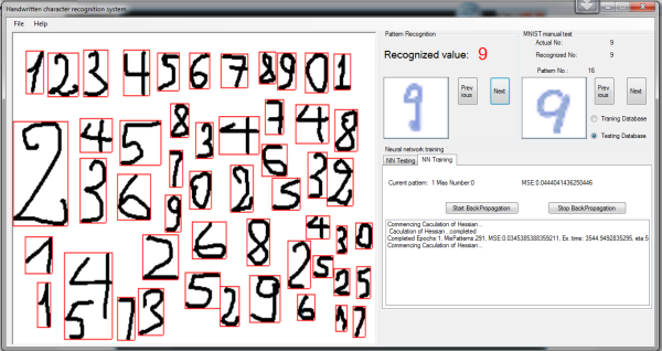
模式检测或字符候选检测是我在程序中面临的最重要的问题之一。事实上,我不仅想用另一种语言简单地重写 Mike 的程序,还想识别文档图片中的字符。我在网上找到了一些研究提出了非常好的对象检测算法,但它们对于像我这样的业余项目来说过于复杂。我在教我女儿画画时找到的一个小算法解决了我的问题。当然,它仍然存在局限性,但在第一次测试中超出了我的预期。通常,字符候选检测分为行检测、单词检测和字符检测,使用不同的算法。我的方法略有不同。通过函数进行相同的检测
public static Rectangle GetPatternRectangeBoundary
	(Bitmap original,int colorIndex, int hStep, int vStep, bool bTopStart)
和
public static List<Rectangle> PatternRectangeBoundaryList
	(Bitmap original, int colorIndex, int hStep, int vStep,
	bool bTopStart,int widthMin,int heightMin)
通过简单地改变参数:hStep (水平步长)和 vStep (垂直步长),可以检测行、单词或字符。通过将 bTopStart 设置为 true 或 false ,也可以从上到下或从左到右检测矩形边界。矩形可以由 widthMin 和 限制。我的算法最大的优点是:它可以检测不属于同一行的单词或字符组。
可以通过以下函数获得字符候选识别
   public void PatternRecognitionThread(Bitmap bitmap)
        {
            _originalBitmap = bitmap;
            if (_rowList == null)
            {
                _rowList = AForge.Imaging.Image.PatternRectangeBoundaryList
		(_originalBitmap,255, 30, 1, true, 5, 5);
                _irowIndex = 0;

            }
            foreach(Rectangle rowRect in _rowList)
            {
                _currentRow = AForge.Imaging.ImageResize.ImageCrop
		(_originalBitmap, rowRect);
                if (_iwordIndex == 0)
                {
                    _currentWordsList = AForge.Imaging.Image.PatternRectangeBoundaryList
			(_currentRow, 255, 20, 10, false, 5, 5);
                }

                foreach (Rectangle wordRect in _currentWordsList)
                {
                    _currentWord = AForge.Imaging.ImageResize.ImageCrop
			(_currentRow, wordRect);
                   _iwordIndex++;
                    if (_icharIndex == 0)
                    {
                        _currentCharsList =
			AForge.Imaging.Image.PatternRectangeBoundaryList
			(_currentWord, 255, 1, 1, false, 5, 5);
                    }

                    foreach (Rectangle charRect in _currentCharsList)
                    {
                        _currentChar = AForge.Imaging.ImageResize.ImageCrop
			(_currentWord, charRect);
                       _icharIndex++;
                        Bitmap bmptemp = AForge.Imaging.ImageResize.FixedSize
			(_currentChar, 21, 21);
                        bmptemp = AForge.Imaging.Image.CreateColorPad
			(bmptemp,Color.White, 4, 4);
                        bmptemp = AForge.Imaging.Image.CreateIndexedGrayScaleBitmap
				(bmptemp);
                        byte[] graybytes = AForge.Imaging.Image.GrayscaletoBytes(bmptemp);
                        PatternRecognitionThread(graybytes);
                        m_bitmaps.Add(bmptemp);
                    }
                    string s = " \n";
                    _form.Invoke(_form._DelegateAddObject, new Object[] { 1, s });
                          If(_icharIndex ==_currentCharsList.Count)
                          {
                          _icharIndex =0;
                          }
                 }
                 If(_iwordIndex==__currentWordsList.Count)
                 {
                          _iwordIndex=0;
                 }
            }
        }
字符识别
原始程序中的卷积神经网络(CNN)本质上是一个具有五个层的 CNN,包括输入层。卷积架构的详细信息已由 Mike 和 Dr. Simard 在他们的文章 "Best Practices for Convolutional Neural Networks Applied to Visual Document Analysis" 中描述。这个卷积网络的一般策略是以更高的分辨率提取简单特征,然后将其转换为更粗糙分辨率下的更复杂特征。生成更粗糙分辨率的最简单方法是将层按因子 2 进行子采样。这反过来又为卷积核的大小提供了一个线索。选择卷积核的宽度是为了以一个单元为中心(奇数大小),具有足够的重叠以不丢失信息(仅一个单元重叠的 3 会太小),但又不会有冗余计算(5 个单元或超过 70% 的重叠的 7 会太大)。因此,在此网络中选择了大小为 5 的卷积核。对输入进行填充(使其更大,以便特征单元位于边界上)并没有显著提高性能。没有填充,子采样为 2,核大小为 5,每个卷积层将特征大小从 n 减少到 (n-3)/2。由于初始 MNIST 输入大小为 28x28,经过 2 层卷积后生成整数大小的 nearest value 是 29x29。经过 2 层卷积后,5x5 的特征大小对于第三层卷积来说太小了。Simard 博士还强调,如果第一层少于五个不同的特征,性能会下降;而使用超过 5 个则不会提高性能(Mike 使用了 6 个特征)。类似地,第二层,少于 50 个特征会降低性能,而更多(100 个特征)则不会提高性能。神经网络的总结如下:
第 0 层:是 MNIST 数据库中手写字符的灰度图像,被填充到 29x29 像素。输入层有 29x29= 841 个神经元。
第 1 层:是具有六 (6) 个特征图的卷积层。有 13x13x6 = 1014 个神经元,(5x5+1)x6 = 156 个权重,以及从第 1 层到前一层的 1014x26 = 26364 个连接。
第 2 层:是具有五十 (50) 个特征图的卷积层。有 5x5x50 = 1250 个神经元,(5x5+1)x6x50 = 7800 个权重,以及从第 2 层到前一层的 1250x(5x5x6+1)=188750 个连接。
(Mike 的文章中不是 32500 个连接)。
第 3 层:是一个具有 100 个单元的全连接层。有 100 个神经元,100x(1250+1) = 125100 个权重,以及 100x1251 = 125100 个连接。
第 4 层:是最终层,有 10 个神经元,10x(100+1) = 1010 个权重,以及 10x101 = 1010 个连接。
反向传播
反向传播是更新每一层权重变化的过程,从最后一层开始,向后穿过各层直到第一层。
在标准反向传播中,每个权重根据以下公式更新:
 (1)
(1)
其中 eta 是“学习率”,通常是一个小的数字,如 0.0005,在训练过程中会逐渐减小。然而,由于收敛速度慢,原始程序不需要使用标准反向传播。取而代之的是,采用了 Dr. LeCun 在其文章 "Efficient BackProp" 中提出的二阶技术,称为“随机对角 Levenberg-Marquardt 方法”。尽管 Mike 说它与标准反向传播没有太大区别,但一点理论知识可以帮助像我这样的新手更容易理解代码。
在 Levenberg-Marquardt 方法中,rw 的计算如下:

假设一个平方成本函数:
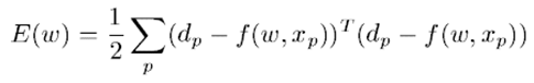
则梯度为:
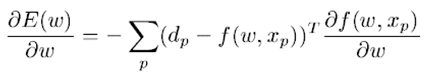
Hessian 矩阵如下:

Hessian 的一个简化近似是 Jacobian 的平方,这是一个 N x O 维度的半正定矩阵。
计算神经网络中对角 Hessian 的反向传播过程是众所周知的。假设网络中的每一层都有函数形式:
![]()
使用 Gaus-Neuton 近似(忽略包含 ¦’’(y) 的项),我们得到:


和

随机对角 Levenberg-Marquardt 方法
事实上,使用完整 Hessian 信息(Levenberg-Marquardt、Gaus-Newton 等)的技术只能应用于批处理模式下训练的非常小的网络,而不是随机模式。为了获得 **Levenberg-Marquardt 算法**的随机版本,LeCun 博士提出了通过对每个参数的二阶导数进行运行估计来计算对角 Hessian 的想法。瞬时二阶导数可以通过反向传播获得,如公式 (7, 8, 9) 所示。一旦我们有了这些运行估计,我们就可以使用它们为每个参数计算单独的学习率:

其中 e 是全局学习率,而  是二阶导数关于 hki 的运行估计。m 是一个参数,用于防止 hki 在二阶导数很小的情况下(即优化函数在误差函数平坦的部分移动时)爆炸。二阶导数可以在训练集的子集(训练集的 500 个随机模式/60000 个模式)上计算。由于它们变化很慢,因此只需要每隔几个 epoch 重新估计一次。在原始程序中,对角 Hessian 每隔一个 epoch 重新估计一次。
这是 C# 中的二阶导数计算函数:
public void BackpropagateSecondDerivatives(DErrorsList d2Err_wrt_dXn /* in */,
                                                    DErrorsList d2Err_wrt_dXnm1 /* out */)
{
    // nomenclature (repeated from NeuralNetwork class)
    // NOTE: even though we are addressing SECOND
    // derivatives ( and not first derivatives),
    // we use nearly the same notation as if there
    // were first derivatives, since otherwise the
    // ASCII look would be confusing.  We add one "2"
    // but not two "2's", such as "d2Err_wrt_dXn",
    // to give a gentle emphasis that we are using second derivatives
    //
    // Err is output error of the entire neural net
    // Xn is the output vector on the n-th layer
    // Xnm1 is the output vector of the previous layer
    // Wn is the vector of weights of the n-th layer
    // Yn is the activation value of the n-th layer,
    //   i.e., the weighted sum of inputs BEFORE the squashing function is applied
    // F is the squashing function: Xn = F(Yn)
    // F' is the derivative of the squashing function
    //   Conveniently, for F = tanh, then F'(Yn) = 1 - Xn^2, i.e.,
    //   the derivative can be calculated from the output,
    //   without knowledge of the input

    int ii, jj;
    uint kk;
    int nIndex;
    double output;
    double dTemp;

    var d2Err_wrt_dYn = new DErrorsList(m_Neurons.Count);
    //
    // std::vector< double > d2Err_wrt_dWn( m_Weights.size(), 0.0 );
    // important to initialize to zero
    //////////////////////////////////////////////////
    //
    ///// DESIGN TRADEOFF: REVIEW !!
    //
    // Note that the reasoning of this comment is identical
    // to that in the NNLayer::Backpropagate()
    // function, from which the instant
    // BackpropagateSecondDerivatives() function is derived from
    //
    // We would prefer (for ease of coding) to use
    // STL vector for the array "d2Err_wrt_dWn", which is the
    // second differential of the current pattern's error
    // wrt weights in the layer.  However, for layers with
    // many weights, such as fully-connected layers,
    // there are also many weights.  The STL vector
    // class's allocator is remarkably stupid when allocating
    // large memory chunks, and causes a remarkable
    // number of page faults, with a consequent
    // slowing of the application's overall execution time.

    // To fix this, I tried using a plain-old C array,
    // by new'ing the needed space from the heap, and
    // delete[]'ing it at the end of the function.
    // However, this caused the same number of page-fault
    // errors, and did not improve performance.

    // So I tried a plain-old C array allocated on the
    // stack (i.e., not the heap).  Of course I could not
    // write a statement like
    //    double d2Err_wrt_dWn[ m_Weights.size() ];
    // since the compiler insists upon a compile-time
    // known constant value for the size of the array.
    // To avoid this requirement, I used the _alloca function,
    // to allocate memory on the stack.
    // The downside of this is excessive stack usage,
    // and there might be stack overflow probelms.  That's why
    // this comment is labeled "REVIEW"

    double[] d2Err_wrt_dWn = new double[m_Weights.Count];
    for (ii = 0; ii < m_Weights.Count; ++ii)
    {
        d2Err_wrt_dWn[ii] = 0.0;
    }
    // calculate d2Err_wrt_dYn = ( F'(Yn) )^2 *
    //    dErr_wrt_Xn (where dErr_wrt_Xn is actually a second derivative )

    for (ii = 0; ii < m_Neurons.Count; ++ii)
    {
        output = m_Neurons[ii].output;
        dTemp = m_sigmoid.DSIGMOID(output);
        d2Err_wrt_dYn.Add(d2Err_wrt_dXn[ii] * dTemp * dTemp);
    }
    // calculate d2Err_wrt_Wn = ( Xnm1 )^2 * d2Err_wrt_Yn
    // (where dE2rr_wrt_Yn is actually a second derivative)
    // For each neuron in this layer, go through the list
    // of connections from the prior layer, and
    // update the differential for the corresponding weight

    ii = 0;
    foreach (NNNeuron nit in m_Neurons)
    {
        foreach (NNConnection cit in nit.m_Connections)
        {
            try
            {
                 kk = (uint)cit.NeuronIndex;
                if (kk == 0xffffffff)
                {
                    output = 1.0;
                    // this is the bias connection; implied neuron output of "1"
                }
                else
                {
                    output = m_pPrevLayer.m_Neurons[(int)kk].output;
                }

                //  ASSERT( (*cit).WeightIndex < d2Err_wrt_dWn.size() );
                // since after changing d2Err_wrt_dWn to a C-style array,
                // the size() function this won't work

                d2Err_wrt_dWn[cit.WeightIndex] = d2Err_wrt_dYn[ii] * output * output;
            }
            catch (Exception ex)
            {

           }
        }

        ii++;
    }
    // calculate d2Err_wrt_Xnm1 = ( Wn )^2 * d2Err_wrt_dYn
    // (where d2Err_wrt_dYn is a second derivative not a first).
    // d2Err_wrt_Xnm1 is needed as the input value of
    // d2Err_wrt_Xn for backpropagation of second derivatives
    // for the next (i.e., previous spatially) layer
    // For each neuron in this layer

    ii = 0;
    foreach (NNNeuron nit in m_Neurons)
    {
        foreach (NNConnection cit in nit.m_Connections)
        {
            try
            {
                kk = cit.NeuronIndex;
                if (kk != 0xffffffff)
                {
                    // we exclude ULONG_MAX, which signifies the phantom bias neuron with
                    // constant output of "1", since we cannot train the bias neuron

                    nIndex = (int)kk;
                    dTemp = m_Weights[(int)cit.WeightIndex].value;
                    d2Err_wrt_dXnm1[nIndex] += d2Err_wrt_dYn[ii] * dTemp * dTemp;
                }
            }
            catch (Exception ex)
            {
                return;
            }
        }

        ii++;  // ii tracks the neuron iterator
    }
    double oldValue, newValue;

    // finally, update the diagonal Hessians
    // for the weights of this layer neuron using dErr_wrt_dW.
    // By design, this function (and its iteration
    // over many (approx 500 patterns) is called while a
    // single thread has locked the neural network,
    // so there is no possibility that another
    // thread might change the value of the Hessian.
    // Nevertheless, since it's easy to do, we
    // use an atomic compare-and-exchange operation,
    // which means that another thread might be in
    // the process of backpropagation of second derivatives
    // and the Hessians might have shifted slightly

    for (jj = 0; jj < m_Weights.Count; ++jj)
    {
        oldValue = m_Weights[jj].diagHessian;
        newValue = oldValue + d2Err_wrt_dWn[jj];
        m_Weights[jj].diagHessian = newValue;
    }
}
//////////////////////////////////////////////////////////////////
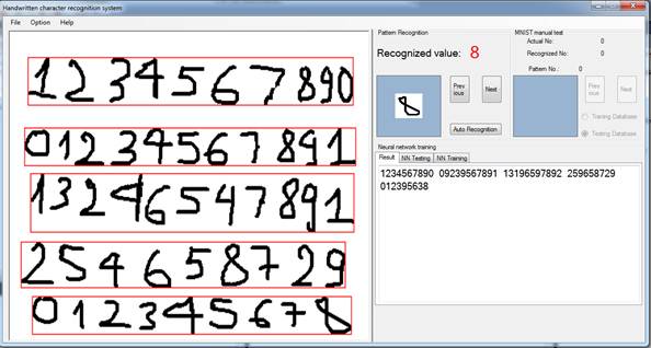
训练和实验
尽管 MFC/C++ 和 C# 之间存在不兼容性,但我的程序与原版相似。使用 MNIST 数据库,网络在训练集的 60,000 个模式中误识别了 291 个,错误率仅为 0.485%。然而,在测试集的 10,000 个模式中误识别了 136 个,错误率为 1.36%。结果不如基准,但足以让我用自己的手写字符集进行实验。首先,输入图片被分割成从上到下的字符组,然后,每个组中的字符将从左到右检测,并调整到 29x29 像素,然后由神经网络识别。该程序总体上满足了我的要求,我的手写数字能够被良好地识别。为了未来的工作,已将检测功能添加到 AForge.Net 的图像处理库中。然而,由于它只是在业余时间编程,所以我确信它存在很多需要修复的 bug。反向传播时间就是一个例子。使用扭曲的训练集,每个 epoch 通常需要大约 3800 秒,而反之则需要 2400 秒。(我的电脑是 Intel Pentium dual core E6500。)与 Mike 的程序等相比,这相当慢。我也希望拥有一个更好的手写字符数据库,或者与他人合作继续我的实验,并为实际应用开发我的算法。


参考文献
- Neural Network for Recognition of Handwritten Digits by Mike O'Neill
- Dr. Yann LeCun 的出版物列表
- Dr. LeCun 网站上关于 "Learning and Visual Perception" 的部分
- 修改后的 NIST(“MNIST”)数据库(总计 11,594 KB)
- Y. LeCun, L. Bottou, Y. Bengio, and P. Haffner, "Gradient-Based Learning Applied to Document Recognition", Proceedings of the IEEE, vol. 86, no. 11, pp. 2278-2324, Nov. 1998. [46 pages].
- Y. LeCun, L. Bottou, G. Orr, and K. Muller, "Efficient BackProp", in Neural Networks: Tricks of the trade, (G. Orr and Muller K., eds.), 1998. [44 pages]
- Patrice Y. Simard, Dave Steinkraus, John Platt, "Best Practices for Convolutional Neural Networks Applied to Visual Document Analysis," International Conference on Document Analysis and Recognition (ICDAR), IEEE Computer Society, Los Alamitos, pp. 958-962, 2003.
- Fabien Lauer, Ching Y. Suen and Gerard Bloch, "A Trainable Feature Extractor for Handwritten Digit Recognition", Elsevier Science, February 2006
- CodeProject.com 上的一些附加项目,这些项目已在本程序中使用: