
关于 ML 和 TensorFlow 的笔记:线性回归
5.00/5 (1投票)
学习机器学习和 TensorFlow 的日记。
引言
线性回归是监督学习中的一个重要算法。在本文中,我将沿用我在参考文献[1](在参考文献部分)中引用的以下表示法:
- xi 表示“输入”变量,也称为输入特征
- yi 表示我们试图预测的“输出”或目标变量
- 一对 (xi, yi) 称为一个训练样本
- 一个包含 m 个训练样本的列表 {xi, yi; i = 1,…,m} 称为一个训练集
- 表示法中的上标“i”(xi 和 yi)是指训练集中的索引
- X 表示输入值的空间,Y 表示输出值的空间。在本文中,我将假设 X = Y = R
- 函数 h: X -> Y,其中 h(x) 是对应 y 值的良好预测器,称为假设或模型
当我们要预测的目标变量是连续的时,我们将该学习问题称为回归问题。当 y 只取少量离散值时,我们称之为分类问题。
背景
在机器学习中,如果我们谈论回归,通常是指线性回归。线性回归意味着您可以将输入乘以某些常数然后相加得到输出,我们将 h 函数表示如下:

其中 wi 是参数(也称为权重),它们参数化了从 X 映射到 Y 的线性函数空间。为了简化,我们还假设 x0 = 1,并且我们的 h(x) 可以表示为:

如果我们同时将 w 和 x 都视为向量,则可以重写 h(x):

其中 x = (x0, x1, x2,…,xn) 且 w = (w0, w1,…,wn)。
到目前为止,一个问题可能会出现:我们如何获得权重 w?为了回答这个问题,我们将定义一个成本函数,该函数用于计算预测 h(x) 与实际 y 之间差异的误差。成本函数如下所示:

我们希望选择 w 以最小化 costF(w)。为此,有两种方法:
- 第一种方法,我们将使用梯度下降算法来最小化
costF(w)。在此方法中,我们反复遍历训练集,每次遇到一个训练样本时,我们都会根据该单个训练样本的误差关于权重的梯度来更新权重。 - 第二种方法,我们将通过显式计算
costF对w的导数并将其设置为零来最小化costF。我们可以将此设置为零并求解w以获得以下方程:

您可以在 [1] 中了解更多关于这些方法的信息。为了在本文中使用代码,我将对第一种方法使用 TensorFlow 库,对第二种方法使用 NumPy 库。
Using the Code
初始化线性模型
在本文中,我假设我们的模型(或 h 函数)是以下方程:
h(x) = w1*x + w0,其中 x0 = 1,x1 = x
初始化训练集
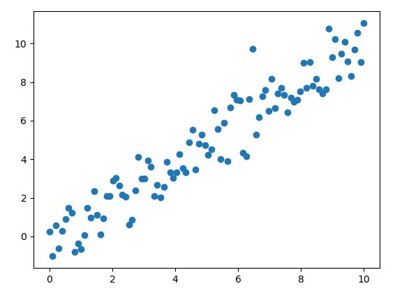
我们需要通过创建以下 Python 脚本来初始化数据:
import numpy as np
import matplotlib.pyplot as plt
# the training set
x_train = np.linspace(0, 10, 100)
y_train = x_train + np.random.normal(0,1,100)
plt.scatter(x_train, y_train)
plt.show()
如果运行此脚本,结果可能如下所示:
梯度下降算法方法
在此方法中,我们反复遍历训练集,每次遇到一个训练样本时,我们都会根据该单个训练样本的误差关于权重的梯度来更新权重。下面的代码将允许您通过使用 TensorFlow 库 为给定的数据创建最佳拟合线:
import tensorflow as tf
import numpy as np
import matplotlib.pyplot as plt
learning_rate = 0.01
# steps of looping through all your data to update the parameters
training_epochs = 100
# the training set
x_train = np.linspace(0, 10, 100)
y_train = x_train + np.random.normal(0,1,100)
# set up placeholders for input and output
X = tf.placeholder(tf.float32)
Y = tf.placeholder(tf.float32)
# Define h(x) = x*w1 + w0
def h(X, w1, w0):
       return tf.add(tf.multiply(X, w1), w0)
# set up variables for weights
w0 = tf.Variable(0.0, name="weights")
w1 = tf.Variable(0.0, name="weights")
y_predicted = h(X, w1, w0)
# Define the cost function
costF = 0.5*tf.square(Y-y_predicted)
# Define the operation that will be called on each iteration
train_op = tf.train.GradientDescentOptimizer(learning_rate).minimize(costF)
sess = tf.Session()
init = tf.global_variables_initializer()
sess.run(init)
# Loop through the data training
for epoch in range(training_epochs):
       for (x, y) in zip(x_train, y_train):
              sess.run(train_op, feed_dict={X: x, Y: y})
# get values of the final weights
w_val_0 = sess.run(w0)
w_val_1 = sess.run(w1)
sess.close()
# plot the data training
plt.scatter(x_train, y_train)
# plot the best fit line
y_learned = x_train*w_val_1 + w_val_0
plt.plot(x_train, y_learned, 'r')
plt.show()
如果我们运行此脚本,结果可能如下所示:

矩阵导数方法
在此方法中,我们将通过显式计算 costF 对 w 的导数并将其设置为零来最小化 costF。您可以使用 TensorFlow 库 中的矩阵方法,但我在这里将使用 NumPy 库 来解决这个问题。下面的代码将允许您通过使用 NumPy 库 为给定的数据创建最佳拟合线:
from numpy import *
import numpy as np
import matplotlib.pyplot as plt
# the training set
x_train = np.linspace(0, 10, 100)
y_train = x_train + np.random.normal(0,1,100)
xArr = []
yArr = []
for i in range(len(x_train)):
       # x0 = 1, x1 = x_train
       xArr.append([1.0,float(x_train[i])])
       yArr.append(float(y_train[i]))
def linearRegres(xArr,yArr):
       xMat = mat(xArr); yMat = mat(yArr).T
       xTx = xMat.T*xMat
       # checking the determination, if you don’t do this, you will get an
       # error when computing the inverse if the determination is zero
       if linalg.det(xTx) == 0.0:
              print("This matrix is singular, cannot do inverse")
              return
       ws = xTx.I * (xMat.T*yMat)
       return ws
# get values of the final weights
w_val = linearRegres(xArr,yArr)
# plot the data training
plt.scatter(x_train, y_train)
# plot the best fit line
y_learned = mat(xArr)*w_val
plt.plot(x_train, y_learned, 'r')
plt.show()
运行上述脚本的结果可能如下所示:

关注点
在本文中,我介绍了解决线性回归问题的两种方法。线性回归的一个问题是它倾向于欠拟合数据,解决此问题的一种方法是称为局部加权线性回归的技术。您可以在 [1] 中找到更多关于此技术的信息。
参考文献
- [1] Andrew Ng 的 CS229 课程笔记
- [2] Peter Harrington 的《机器学习实战》
- [3] Nishant Shukla 的《使用 TensorFlow 进行机器学习》
- [4] Nick McClure 的《TensorFlow 机器学习宝典》
- [5] Joel Grus 的《从零开始的数据科学》
- [6] Aurélien Géron 的《使用 Scikit-Learn 和 TensorFlow 进行机器学习实战》
历史
- 2019年4月21日:初版