
QR 分解真的能更快吗?Schwarz-Rutishauser 算法
5.00/5 (11投票s)
使用 Schwarz-Rutishauser 算法优化大型矩阵的 QR 分解和特征值分解的性能
- 下载 qr_eigen_factorization.zip - 14.8 KB
- 下载 2021_12_19_16_46_56_1720x1448.mp4 - 331.7 KB
- 下载 2021_12_19_16_40_16_1720x1448.mp4 - 315.1 KB
- 下载 2021_12_19_16_36_24_1720x1448.mp4 - 751.3 KB
目录
引言
QR 分解是最新的、也是可能是最有趣的线性代数算子之一,它在科学和工程的许多领域都有多种已知应用。QR 分解的相关研究始于 20 世纪初。一整类 QR 分解算法在数学中被有效地用于解决线性最小二乘 (LS) 问题、求解线性方程组、降低各种矩阵的维度,以及作为特征值计算和奇异值分解 (SVD) 方法 [1] 的关键步骤等。
在过去的几十年里,计算机科学和 IT 领域的蓬勃发展影响了研究人员对最优大型矩阵 QR 分解方法日益增长的兴趣,这是解决许多现实世界问题(由现代计算机解决)的算法中的一个关键步骤和子过程。
- 图像和数字摄影的变换,包括旋转、增强、扭曲和 3D 透视,同时解决 SVD 问题,其中 QR 分解是关键步骤。基于 SVD 算法实现的以下形状变换过滤器,常用于各种图形应用程序,如 Adobe Photoshop、Affinity Photo 和 GIMP 等。
- 通过几种基于插值的方法确定电信号的唯一(即“奇异”)特征,这些方法广泛用于数字信号处理,以识别噪声和其他伪影,从而能够恢复由失真信号引起的损坏数据。所有这些方法都基于向量正交性质。为了找到信号有影响力的异常特征,将每个参数值的集合分解为多个局部子集。以下分解被计算为每个参数向量在希尔伯特空间 ℋ [2] 中的相应轴上的正交投影。许多现有的异常和伪影分析方法依赖于向量正交投影,这可以很容易地基于 QR 分解方法进行计算。
- 利用多种主成分分析 (PCA) 方法分析工业机器和机械的振动水平,这些方法用于将多个参数表示为可能具有解释性的因子,以检测振动和声学环境干扰 [15]。
- 从大型统计数据集中获取知识和见解,以找到能够理解哪些因素对各种经济因素(如销售额、年度股市收盘价以及交易公司进行的其他估计)产生最关键影响的趋势,从而有效地把握业务,旨在提高全球数十亿在线客户所销售的商品、数字内容和服务的受欢迎程度并降低潜在成本 [1,3,16]。在这种情况下,QR 分解方法被用作数据归一化技术,消除数据集中各种冗余且无信息量的数据,从而提供对所揭示的统计知识和趋势的更好理解。
此外,QR 分解过程会产生正交因子矩阵,这是一种特殊的函数矩阵,其中最常见或最相似的因子值被聚合到多个区域。矩阵分解在解决各种分类问题时,在有效数据聚类方面具有优势。它被用作许多基于 AI 的监督学习算法的替代方案,执行基于大型数据集和连续学习的聚类。
如今,有多种线性代数方法广泛用于执行实数或复数矩阵的 QR 分解,包括改进的 Gram-Schmidt 过程、Householder 反射或 Givens 旋转。
这些方法各有优缺点。改进的 Gram-Schmidt 和 Householder 反射对于复数矩阵分解来说“很重”,而 Givens 旋转方法在其最后几次迭代中会产生精度损失,因此对于大型矩阵效率不高。
在本文中,我将重点讨论 20 世纪 60 年代中期 Schwarz 和 Rutishauser 提出的改进 Gram-Schmidt 正交化方法的优化。为了展示其效率,我使用 Python 3.6 开发了具体的代码和演示应用程序,实现了改进的 Gram-Schmidt、Householder 反射和 Schwarz-Rutishauser 算法 [1,4],并对 Schwarz-Rutishauser 算法与讨论的另外两种方法相比的速度提升进行了调查。
背景
QR 分解基础知识
首先,我们简要回顾一下 QR 分解的过程。它假定整个 QR 分解过程依赖于将任何实数或复数矩阵 A 分解为正交矩阵 Q 和上三角矩阵 R 的乘积,如下所示:

从几何上看,方阵 Q 是一个面向列的多向量,其向量构成 A 的正交基。反过来,第二个矩阵 R ,形状任意,是一个上三角旋转矩阵,它与 Q 中的列向量相乘,将每个向量在 ℝn 空间坐标中旋转 90 度。这通常会导致 Q 中的每个向量都与 A 中的相应向量正交,从而形成其标准正交基。
因此,我们的目标是计算出矩阵 Q 和 R ,使得它们的乘积近似等于给定矩阵 A ,如下所示:

找到正交矩阵 Q 是最关键的步骤。可以通过几种已知的方法获得矩阵 Q ,例如:
- 改进的 Gram-Schmidt 过程
- Householder 反射
- Givens 旋转
通常,正交 Q 的计算会产生矩阵 A 的分解 [1,4]

正交化后的矩阵 Q 可以得到 A 的分解 [4],因此存在满秩分解和部分秩分解。QR 分解不仅可以应用于方阵,还可以应用于矩形矩阵,即使矩阵不是满秩的。通常,A 的满秩分解会得到一个列数与 A 相同的矩阵 Q [5]。A 的分解是一种有用的特性,当 A 中的值必须表示为其因子时,就会应用它 [1,3]。
在获得矩阵 Q 时,它的每个列向量都与之前计算出的其他向量的跨度正交。这些列向量构成了 A 的标准正交基,这与将 ℝⁿ 欧几里得空间中的每个向量映射到 ℝ’ⁿ 空间的不同坐标系相同。“标准正交”意味着 Q 中所有正交列向量都已归一化,除以它们的欧几里得范数 [1,2,6]。
由于我们已经得到了正交的 Q ,第二个矩阵 R 可以通过 Q 的转置与给定矩阵 A 相乘得到 (1.1)

结果矩阵 R 是一个下三角元素全部为 0 的矩阵。具体来说,R 的计算导致对 A 进行高斯消元,将其约化为行阶梯形 [1,4,5,6]。在这种情况下,标量元素 rᵢₖ 和 rₖₖ 乘以希尔伯特空间 ℋ [2] 的子空间单位基向量 eₖ 。通常,这会导致 R 中那些元素与对角元素相抵消。
根据其定义,希尔伯特空间是一种基本类型的欧几里得空间,其向量具有正交和共线性。此外,可以对这些向量应用各种线性代数运算,包括向量与旋转矩阵的标量乘法,这会导致向量旋转,将其旋转到特定角度,从而将其映射到另一个欧几里得空间的不同坐标系。
上面提到的上三角矩阵 R 可以有效地用于求解线性最小二乘 (LS) 问题,以及找到 Ax=b 线性方程组的唯一非平凡解 [1],这是计算 A 的特征值和特征向量,即 A 的特征值分解的基础。
矩阵 R 必须是上三角形式,并且每一列中对应对角元素之后的元素都必须被消去为 0。
最后,矩阵 Q 必须满足正交条件 (1.2),如下所示,因此 Q 是一个正交矩阵,使得 Q 的转置与 Q 的乘积始终等于或近似等于一个在对角线上为 1 的单位矩阵 I

如果满足上述条件,则矩阵 Q 是正交的,并且已正确计算。它用作验证技术,以确定 A 是否已正确正交化。同时,条件 (1.2) 也是 QR 分解算法的停止准则。
此外,根据方程 (1.1) 和 (1.2) ,还可以计算出特征值矩阵 E 和特征向量矩阵 Ѵ 。通常通过获得矩阵 R 和 Q 的乘积来找到特征值 E=diag{eᵢ ∈ E}

或者,也可以通过计算 Q 的转置、A 和 Q 的乘积来计算特征值,如下所示:

使用上面的方程,在进行基于迭代方法的分解时,可以获得更好的特征值分解 QR 算法收敛性。
基本上,为了计算特征值 E 和相应的正交特征向量 Ѵ ,应用了“简单迭代法”。此方法将在本文后续段落 计算特征值与特征向量 (QR 算法) 中进行详细讨论。
一个平凡的 3x3 实数矩阵 A 的 QR 分解可以表示为:
最初,我们有一个整数值的方阵 A (3x3):

矩阵 A 具有三个列向量 a₁(7;-5;4)、a₂(3;8;7)、a₃(1;3;-6),分别用(红色)、(蓝色)和(绿色)表示,投影在三维欧几里得空间 ℝ³ 的坐标中,如下面图所示:
通过执行上述讨论的多向量 A 的 QR 分解后,我们得到两个矩阵 Q 和 R 。第一个矩阵 Q 包含三个正交向量 q₁(-0.73; 0.52; -0.42)、q₂(-0.20; -0.77; -0.59)、q₃(-0.64; -0.35; 0.68),每个向量都有一个相应的 A 中的向量,如下所示:
Q 向量
在这种情况下,Q 中的所有正交向量形成一个标准正交基,它是多向量 A 的分解。正如我们已经讨论过的,A 的任何正确分解都必须满足条件:每个正交向量 qᵢ 必须与其他先前计算出的向量正交(即垂直)。这些向量之间的夹角始终为 90°,并且它们的标量点积近似等于 0,例如 (qᵢ₋₁ · qᵢ ≈ 0)。如果任何先前向量与当前向量 qᵢ ∈ Q,i=1..n 的乘积等于 0,则表示它是矩阵 A 的正确分解。每个归一化向量 qᵢ ∈ Q 的长度 |q| 必须属于区间 |q| ∈ (0;1)。
这里是证明
在这种情况下,Q 中的所有向量 qᵢ ∈ Q,i=1..n,如图所示,与 A 中的向量 aᵢ ∈ A,i=1..n 具有相同的颜色。最初,第一个向量 q₁(-0.73; 0.52; -0.42) 是向量 a₁(7;-5;4) 的归一化对应向量:
|a₁| = √7²+(-5)²+4²=√49+25+16=√90 = 9.4868
q₁=(-(7÷9.4868); -(-5÷9.4868); -(4÷9.4868))=(-0.73; 0.52; -0.42)
我们需要计算向量 a₁ 的欧几里得范数,然后用其范数 |a₁| 除以向量 q₁ 的每个分量。
下一个向量 q₂(-0.20; -0.77; -0.59) 与 q₁(-0.73; 0.52; -0.42) 正交,因为它们的标量积 (q₁ · q₂) 等于 0。
q₁ · q₂ = (-0.7379)⋅(-0.209)+0.527⋅(-0.7724)+(-0.4216)⋅(-0.5998) = 0.1542±0.4071+0.2529 = 0
对向量 q₂(-0.20; -0.77; -0.59) 和 q₃(-0.64; -0.35; 0.68) 也可以进行相同的计算。
q₂ · q₃ = (-0.6418)⋅(-0.209)+(-0.3544)⋅(-0.7724)+0.6801⋅(-0.5998) = 0.1341+0.2737±0.4079 = 0
最后,向量 q₁ · q₃ 也正交,因为它们的标量积近似等于 0。
q₁ · q₃ = (-0.7379)⋅(-0.6418)+0.527⋅(-0.3544)+(-0.4216)⋅0.6801 =0.4736±0.1868±0.2867 = 0.0001 ≈ 0
从上面的计算可以看出,所有向量 q₁、q₂、q₃ 都是正交的,因此多向量 A 的分解是正确的。或者,通过计算矩阵 Q 的转置与 Q 的内积来进行相同的正交性检查,该内积始终是一个单位矩阵 I,其对角线元素为 1。
与正交的 Q 不同,矩阵 R 的向量不是正交的。这些向量是通过标量乘法将 Q 中的每个列向量 qₖ ∈ Q 与 Q(k) 中先前获得的向量跨度中的相应向量 qᵢ 相乘而逐列得到的。这些向量的乘积产生对角元素 rᵢₖ = qᵢ · qₖ 的值,然后将其乘以希尔伯特空间 ℋ [2] 的每个子空间的单位基向量 e₁=(1;0;0)、e₂=(0;1;0) 和 e₃=(0;0;1),以消除 R 的 i 行和 k 列中与相应对角元素 rᵢₖ 相抵消的所有元素。最初,对角元素 r₁ ∈ R 简单地通过 Q 中第一个列向量 q₁ 的范数 |q₁| 得到,即 r₁=|q₁|。此向量运算在用于 Schwarz-Rutishauser 方法时进行,并且与改进的 Gram-Schmidt 正交化方法中 Q 的转置或其共轭与多向量 A 的乘法非常相似。最后,我们将在上三角矩阵 R 的每一行中得到结果向量 r₁(-9.48; -0.94; 3.37)、r₂(0; -11; 1.07) 和 r₃(0; 0; -5.78):
R 向量
上述向量标量乘法导致多向量 A 的高斯消元变为行阶梯形。结果矩阵 R 提供方程系统 A 的唯一非平凡解,避免了复杂的逆矩阵运算。
矩阵的特征值分解
方阵的特征值分解是 QR 分解最有效的应用之一。通过执行矩阵 A 的特征值分解,我们将得到一个特征值向量和一个特征向量矩阵,分别为 E 和 Ѵ 。QR 算法是求解 A 的特征值分解的第一种方法 [7]。
在几何上,矩阵 A 的特征值可以很容易地通过矩阵 R 和 Q 的乘积获得,如上所述。或者,A 的特征值可以作为矩阵 Q 的转置、A 和 Q 的乘积来计算 [8]。
在大多数情况下,Q 的转置乘以 A 和 Q 会得到一个对角线元素为特征值 eᵢ ∈ diag{E} 的结果矩阵 E 。如上所述,获得这个乘积与将旋转矩阵 R 乘以正交矩阵 Q 非常相似,这会导致 Q 的每个向量逆时针旋转,从而使 Q 中的所有向量与被分解的矩阵 A 的列向量“垂直”,因此“正交”。在被 R 旋转时,Q 中每个列向量的长度(即“幅度”)被拉伸。最后,向量 qᵢ ∈ Q 被拉伸的长度程度是向量 aᵢ ∈ A 的相应特征值 eᵢ [10]。
特征向量矩阵 Ѵ 可以通过计算矩阵 Ѵ 和 Q 的内积来计算,得到新的矩阵 Ѵ 。最初,矩阵 Ѵ 只是一个单位矩阵,其对角线元素为 1 [10,11,12]。
根据 QR 算法,结果矩阵 E 和 Ѵ 是迭代计算的,以逼近结果的特征值和特征向量矩阵。使用 QR 算法可以计算出矩阵 E 和 Ѵ ,最多需要 ~ O(30 x n) 次迭代,其中 n 是 A 的列数 [8,9]。
特征值与特征向量计算 (QR 算法)
矩阵 A 的特征值 E 和特征向量 Ѵ 可以基于下面讨论的 Schur 矩阵分解算法轻松计算。整个 QR 算法很简单,可以表述如下 [8,9]:
1. 通过求解 Schur 分解计算 A 的实特征值,** 使用迭代算法;
2. 通过求解 A 的对角子矩阵多项式(即二次方程)来计算 A 的复特征值;
3. 通过 Jordan-Gaussian 方法将 A 约化为行阶梯形并通过求解线性方程组来计算 A 的特征向量;
下面列出了实现 QR 算法的代码片段:
def qr_eig_solver(A, n_iters, qr):

    # Do the simple QR-factorization to compute the 'real' eigenvalues of A
    E = qr_simple(A, n_iters, qr)

    # Solve the polinomial for each diagonal sub-matrix E'
    # to obtain the 'complex' eigenvalues of A
    E = qr_eig_vals_complex_rt(E)

    # Sort the eigenvalues in the ascending order
    E = np.flip(np.sort(E))

    # Compute the eigenvectors V of A, solving the linear equation system,
    # eliminating A to row-echelon form using the Jordan-Gaussian method
    V = qr_eig_vecs_complex_rt(A, E)

    return E, V                     # Return the resultant vector E and matrix V
步骤 #1:计算“实”特征值 eᵢ ∈ ℝⁿ:
首先,我们必须计算 A 的 ℝⁿ 域的“实”特征值。这通常通过使用基于迭代的方法完成,该方法依赖于在 d 次迭代内求解 QR 分解。最初,它将矩阵 A 赋值给结果矩阵 E (E=A)。为了计算 A 作为 E 中对角元素的特征值,它执行 d 次迭代。在每次 i 次迭代中,它计算 A 的相同 QR 分解,得到结果矩阵 Q 和 R。然后,它通过 R 和 Q 的内积计算对角矩阵 E,迭代地逼近 E 中对角元素的近似值。最后,在每次迭代结束时,特征值矩阵 E 被赋值给新矩阵 A。它继续进行下一个 (i+1) 次迭代,计算 A 的相同分解,并得到结果矩阵 E,直到 E 中的所有对角元素都是 A 的特征值 [8,9]。
整个“迭代算法”非常简单,可以表述如下:
1. 初始化矩阵 E,使其等于 A (E=A);
2. 执行 d 次迭代 i=𝟏..d,并执行以下操作:
2.1. 计算矩阵 E 的 QR 分解,即 [Q, R]=QR(E);
2.2. 通过计算 Q 的转置、E 和 Q 的乘积来计算新矩阵 E;
3. 返回“实数 A 的特征值”矩阵 E;
下面列出了说明迭代 QR 算法实现的的代码片段:
def qr_simple(A, n_iters, qr):

    # Initialization: [ E - a square (n x n) matrix of eigenvalues E = A ]
    E = np.array(A, dtype=float)

    # Do n_iters x n - iterations to compute the 'real' eigenvalues of A:
    for i in range(np.shape(A)[1] * n_iters):
        Q,R = qr(E, float);                      # Solve the QR-decomposition of E at i-th iteration
        E = np.transpose(Q).dot(E).dot(Q)        # Compute the product of Q's-transpose, E and Q as the new matrix E

    return E                                     # Return the resultant matrix of 'real' eigenvalues E
步骤 #2:计算“复数”特征值 eᵢ ∈ ℂⁿ:
除了 A 的“实”特征值之外,它还计算“复数”特征值 eᵢ ∈ ℂⁿ,如果存在。为此,它从前一步得到的矩阵 E 的对角线上的每个 2x2 子矩阵 E* 的多项式中获得复数根。每个子矩阵 E* 的多项式的根是一对复数特征值 e'₁₁ 和 e'₂₂。由于每个对角子矩阵 E* 的秩为 2,我们只需要求解一个二次方程,该方程可以写成 [12,14]:

其中,λ 是 2x2 子矩阵的特征值,tr(E* ) 是 E* 的对角元素之和,det(E* ) 是 E* 的行列式。
为了求解上述方程,我们首先需要得到两个子矩阵 E* 的对角元素之和的平均值 μ=avg{diag{eᵢ ∈ E* }},以及其行列式 ρ=det(E* ),最后将 μ 和 ρ 的值代入以下公式:

求解方程后,两个复数根 λ₁ 和 λ₂ 分别赋值给矩阵 E 的对角元素 e₁₁ 和 e₂₂。对 E 的每个 i 阶对角子矩阵重复此过程,直到最终计算出 E 对角线上的 ℂ² 域的所有复数特征值 eᵢ ∈ E。
最后,将步骤 1 中的“实”特征值和 A 的“复数”特征值合并到 A 的特征值结果向量中。
def qr_eig_vals_complex_rt(E):

    n = np.shape(E)[1]                    # Get the number of columns in E

    if n >= 2:                            # Check if the number of columns is >= 2

        es = np.zeros(n, dtype=complex)   # Initialize the array of complex roots

        i = 0

        # For each diagonal element E[i][i], solve the i-th polynomial:
        while i < n - 1:

            # Calculate the sub-matrix E[i:i+1,i:i+1]'s diagonal elements mean
            mu = (E[i][i] + E[i+1][i+1]) / 2

            # Obtain the determinant of the sub-matrix E[i:i+1,i:i+1]
            det = E[i][i] * E[i+1][i+1] - E[i][i+1] * E[i+1][i]

            # Take the complex square root of mu^2, subtracting the determinant of E[i:i+1,i:i+1],
            # to solve the diagonal sub-matrix's of rank ^2 polynomial (i.e., quadratic equation)
            dt_root = cmath.sqrt(mu**2 - det)

            # Compute the eigenvalues e22 and 33, by subtracting the complex square root value
            # from the average of diagonal elements in the sub-matrix es[0:2,0:2],
            # and place them along the sub-matrix es[0:2,0:2]'s diagonal
            e1 = mu + dt_root; e2 = mu - dt_root

            # If e1 is complex, add e1 and e2 to the array es
            if np.iscomplex(e1):
               # If real parts of e1 and e2 are equal, conjugate e2
               if e1.real == e2.real:
                  e2 = np.conj(e2)

               # Append the pair of eigenvalues e1 and e2 to the array es
               es[i] = e1; es[i+1] = e2

               # Sort up the eigenvalues e1 and e2 in the ascending order
               if es[i] < es[i+1]:
                  es[[i]] = es[[i+1]]

               i = i + 1

            i = i + 1

    E = np.diag(E)                         # Extract 'real' eigenvalues from the E's diagonal

    # Combine two arrays E and es of the 'real' and 'complex' eigenvalues
    es = [E[i] if i in np.argwhere(es == 0)[:,0]
            else es[i] for i in range(n)]

    return es                              # Return the resultant array of eigenvalues
步骤 #3:计算 A 的特征向量
最后一步是通过求解 A 的线性方程组,将矩阵 A 约化为行阶梯形,使用 Jordan-Gaussian 消元来计算 A 的特征向量。这通常通过为每个特征值 ek ∈ E 求解 n 个线性方程组,并从 A 的最后 n 列中提取相应的特征向量 vk 来完成。如果 ek ∈ ℂⁿ 是复数,则 A 的最后一列逆时针旋转 90 度,以获得 A 的第 k 个复特征向量 vk ∈ Ѵ [13,14]。
令 A 为形状为 (n x n) 的“实”或“复数”方阵,E 为 A 的 n 个特征值组成的向量。
对于 A 的每个特征值 ek ∈ E,k=1..n,使用 Jordan-Gaussian 方法求解线性方程组:
1. 从 A 的每个对角元素 ajj ∈ A 中减去第 k 个特征值 ek,即 ajj = ajj - ek;
2. 对于每一行 aᵢ ∈ A,i=1..n,进行如下的行阶梯形消元:
2.1. 确定第 i 个基元素 αᵢ = aᵢᵢ;
2.2. 检查 αᵢ 的值是否为 0 或 1。如果是,则将第 i 行 aᵢ ∈ A 中的每个元素除以基元素 αᵢ:aᵢ = aᵢ / αᵢ,否则继续执行下一步 2.3;
2.3. 检查 αᵢ 的值是否为 0。如果是,则交换 A 中的第 i 行和第 (i+1) 行,或者继续执行下一步,除非另有指示;
2.3. 对于除了 aᵢ (j ≠ i) 之外的每一行 aj ∈ A,j=1..n,获取其基元素 Θ = ajj,然后重新计算其元素值 aj,r = aj,r,其中:aj,r = aj,r - aᵢk * Θ;
2.4. 检查 aᵢ 是否是 A 的最后一行,即 i = n。如果不是,则返回步骤 2.1,否则继续执行下一步;
2.5. 将 1.0 赋值给 A ∈ A 的最后一个对角元素 ann,即 ann=1.0;
3. 将最后 n 列 an ∈ A 中的所有元素值提取为 A 的第 k 个特征向量 vk ∈ Ѵ;
4. 通过将其除以向量的欧几里得范数 |vk| 来归一化特征向量 vk ∈ Ѵ;
5. 如果第 k 个特征值 ek ∈ ℂⁿ 是复数,则将每个复数值 vki ∈ Ѵ 旋转 90 度,即:

下面列出了说明 A 的特征向量计算的代码片段:
def rot_complex(val):

    # Rotate the val's 'real' part by the 90-degree angle, counter clockwise
    v_rr = val.real * math.cos(math.pi / 2) + val.imag * math.sin(math.pi / 2)
    # Rotate the val's 'imaginary' part by the 90-degree angle, counter clockwise
    v_ri = val.real * math.sin(math.pi / 2) + val.imag * math.cos(math.pi / 2)

    return v_rr + 1.j * v_ri        # Return the new orthogonal complex value in the space C'n

def qr_eig_vecs_complex_rt(A, E):

    (m,n) = np.shape(A)

    V = np.identity(n, dtype=complex)

    # Compute eigenvectors of A by solving the quadrant polynomial
    # ============================================================

    # Reduce the matrix A to the Jordan-Gaussian row-echelon form:
    #   For each eigenvalue e in E and column-vector in V do the following:
    for (e,z) in zip(E, range(m)):

        Av = np.array(A, dtype=complex)

        # Subtract the eigenvalue e from each diagonal element in Av
        #np.fill_diagonal(Av, np.array([ a - e for a in np.diag(Av)], dtype=complex))

        for j in range(m):
            Av[j][j] = Av[j][j] - e

        # For each i-th row in Av do the following:
        for i in range(m-1):

            # Get the i-th row's basis element alpha
            alpha = Av[i][i]

            # If alpha is not 0 or 1 divide each element in i-th row of Av
            # by the row's basis element alpha,to get 1 at the position of alpha
            if alpha != 0 and alpha != 1:
               #Av[i] = np.array([Av[i][j] / alpha for j in range(m)], dtype=complex)
               for j in range(m):
                   Av[i][j] = Av[i][j] / alpha

            # If alpha is already 0 (in 'rare' case), exchange i-th and (i+1)-th rows of Av
            Av[[i, i+1]] = Av[[i+1, i]] if alpha == 0 else Av[[i, i+1]]

            # For each row in Av, do the row-echelon elimination
            # This turns its basis element alpha into 0 of each column in Av
            for k in range(m):

                theta = Av[k][i]            # Get the diagonal element theta

                if i != k: # If is this *NOT* the current i-th row in Av (i != k), eleminate alpha for i-th row
                #Av[k,i:] = np.array([Av[k][j] - Av[i][j] * theta for j in range(i,m)], dtype=complex) if i != k else Av[k,i:]
                   for j in range(i,m):
                       Av[k][j] = Av[k][j] - Av[i][j] * theta

        # Since the last (m-1)-th column of Av is the current eigenvector in V
        # Copy the (m-1)-th row to z-th column of V, assigning 1.0 to its last (m-1)-th element
        V[:,z] = Av[:,m-1]; V[m-1][z] = 1.0

        # Obtain the Euclidean norm of z-th column in V
        nV = lin.norm(V[:,z])
        # Norm the z-th eigenvector in V by dividing each of its elements by the norm nV
        V[:,z] = np.array([v / nV for v in V[:,z]], dtype=complex)

        # If eigenvalue e is complex, rotate the corresponding
        # eigenvector counter clockwise by 90-degree angle
        V[:,z] = [rot_complex(v) for v in V[:,z]] if e.imag != 0 else V[:,z]

        z = z + 1

    return V
关于计算奇异值分解 (SVD) 的简要说明
计算 SVD(奇异值分解)是执行 QR 分解并找到实数或复数矩阵 A 的特征值和特征向量的下一个重要步骤。
SVD 计算通常在目标是获得方阵 A 在其标准正交特征空间中的分解时应用,该分解揭示了最常见的潜在或解释性因素,同时解决了各种数据分类和聚类问题,以及在声学水平分析或数字信号处理等许多科学和工程过程中寻找参数中的奇异值,如上所述。
显然,A 分解为奇异值对角矩阵 Σ 以及左奇异向量 U 和右奇异向量 V 可以表示为:

根据此,SVD 是矩阵 A 分解为左奇异向量矩阵 U、奇异值对角矩阵 Σ 和右奇异向量矩阵 V 的转置的内积。
SVD 分解的求解分几个步骤完成,如下所示:
步骤 #1:获得 A 的对称矩阵 AᵗA
正确求解 SVD 分解的前提是,给定的矩阵 A 是一个对称矩阵,我们旨在计算其奇异值和向量,执行 A 的分解。在这种情况下,A 的对称矩阵是通过 A 的转置与 A 的乘积计算得出的,即:

如您所见,对称矩阵 A' 是通过 A 的转置乘以 A 得到的,在大多数情况下,这是一个方对称矩阵。计算矩形矩阵的对称矩阵是不可能的,因此,矩形矩阵的 SVD 分解通常无法求解。
既然我们已经获得了 A 的对称矩阵,让我们继续进行下面的 SVD 分解步骤。
步骤 #2:计算奇异值对角矩阵 Σ:
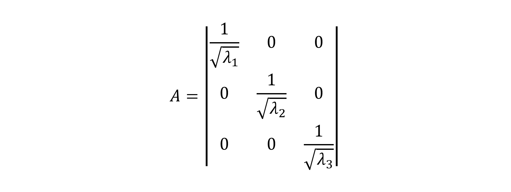
SVD 分解算法完全依赖于矩阵 QR 分解,该分解可以得到对角特征值矩阵 E 以及相应特征向量矩阵 Ѵ 。A 的特征值和特征向量的特定计算方法已在上面讨论过。为了计算对角奇异值矩阵 Σ,将每个特征值 eᵢ ∈ E,i=1..n 的平方根取值并放置在 Σ 矩阵的对角线上,得到 Σ 的逆矩阵,如下所示:

在这里,Σ 中的所有特征值也必须按升序排列,从最大的特征值开始,赋值给第一个对角元素 s₁₁=max{eᵢ ∈ E}。得到的逆矩阵 Σ⁻¹ 是通过将 1.0 除以每个对角元素 sᵢᵢ ∈ Σ 得到的,如下所示:
最后,逆矩阵 Σ⁻¹ 中的所有对角元素将成为 AᵗA 的奇异值。
既然我们已经计算出了 AᵗA 的奇异值矩阵 Σ=Σ⁻¹,我们就继续进行下面段落中讨论的左奇异向量和右奇异向量的计算。
步骤 #3:计算 AᵗA 的右奇异向量
AᵗA 的右奇异向量通常是通过求解给定特征值对角向量 e = diag{eᵢ ∈ E} 和具有 1 作为对角元素的单位矩阵 I 的线性方程组的唯一非平凡解来获得的:

上述线性方程组的非平凡解基本上是通过使用著名的 Jordan-Gaussian 消元方法找到的,该方法将矩阵 AᵗA 降至行阶梯形,从而获得上三角矩阵 AᵗA。
然后,通过使用以下公式,将每个右奇异向量除以向量的绝对标量长度 L 来归一化:

之后,右奇异向量 vᵢ ∈ V,i=1..m 沿矩阵 V 的相应行放置,并将 V 转置,因此 Vᵗ 最终成为矩阵 A 的右奇异向量矩阵。
步骤 #4:计算 AᵗA 的左奇异向量
由于我们已经计算出奇异值矩阵 Σ 和 Vᵗ,现在我们可以计算 A 的左奇异向量矩阵 U,这通常是通过计算矩阵 A、Vᵗ 和对角矩阵 Σ 的乘积来完成的,如下所示:

以下计算结果是获得 A 的左奇异向量矩阵 U,其所有奇异向量都在 U 的列中。
最后,让我们进行验证,以确定 A 的 SVD 分解是否已正确完成。与 QR 分解类似,这是通过计算 U、Σ 和 Vᵗ 的乘积来完成的,该乘积始终必须近似等于给定矩阵 A。
在我之前的一篇文章 《C++11 中的奇异值分解 (SVD) 示例》 [《Singular Values Decomposition (SVD) In C++11 By An Example》, Arthur V. Ratz, CodeProject, November 2018] 中,对求解奇异值分解 (SVD) 的过程进行了详细讨论,并说明了具体的 SVD 计算步骤。
改进的 Gram-Schmidt 正交化
Gram-Schmidt 过程是在 20 世纪 50 年代中期提出的,是第一个成功用于实数或复数矩阵正交化的方法 [1,4,5,6]。这是计算给定矩阵 QR 分解的最简单方法。其他方法,例如基于镜面反射的 Householder 反射,通常更复杂。因此,让我们首先简要讨论改进的 Gram-Schmidt 正交化方法,然后再解释 Schwarz-Rutishauser 算法。
该方法主要用于递归地找到 A 的 Q 矩阵,基于将每个向量 aₖ ∈ A,k=1..n 正交投影到已计算向量 qᵢ ∈ Q(k),i=1..k 的跨度上。每个新的正交向量 qₖ ∈ Q 是通过从相应向量 aₖ ∈ A 中减去每个先前找到的正交投影的总和来计算的。另一个上三角矩阵 R 可以通过 Q 的转置与矩阵 A 相乘得到,如方程 (1) 所示。根据改进的 Gram-Schmidt 方法,在寻找 Q 的相应列向量时,A 的每一行到 R 的高斯消元通常是就地进行的。
使用方程 (2):计算 a 到 q 的正交投影,如下所示:

通常,改进的 Gram-Schmidt 过程会产生 Q 矩阵的计算,该计算可以代数表示为:

或者,备选地:

每个新向量 qₖ ∈ Q 最终通过除以其欧几里得范数 |qₖ| 进行归一化。
下面列出的 Python 代码片段实现了改进的 Gram-Schmidt 正交化过程。
def conj_transpose(a):
    return np.conj(np.transpose(a))

def proj_ab(a,b):
    return a.dot(conj_transpose(b)) / lin.norm(b) * b

def qr_gs(A, type=complex):
    A = np.array(A, dtype=type)
    (m, n) = np.shape(A)

    (m, n) = (m, n) if m > n else (m, m)

    Q = np.zeros((m, n), dtype=type)
    R = np.zeros((m, n), dtype=type)

    for k in range(n):
        pr_sum = np.zeros(m, dtype=type)

        for j in range(k):
            pr_sum += proj_ab(A[:,k], Q[:,j])

        Q[:,k] = A[:,k] - pr_sum
        Q[:,k] = Q[:,k] / lin.norm(Q[:,k])

    if type == complex:
        R = conj_transpose(Q).dot(A)
    else: R = np.transpose(Q).dot(A)

    return -Q, -R
改进的 Gram-Schmidt 正交化过程存在一些缺点,例如数值不稳定,以及应用于大型矩阵时计算复杂度相当高,高达 O(2mn²)。此外,在分解矩形 m x n 矩阵时,它需要修改以确定矩阵的领先维度 [4]。
Schwarz-Rutishauser 算法
正如你可能已经注意到的,这里讨论的 Schwarz-Rutishauser 算法完全基于改进的 Gram-Schmidt 正交化,其复杂度通常很高,这是由于计算每个向量 aₖ ∈ A 到 qᵢ ∈ Q(k) 的投影所致。因此,我们需要一种稍微不同的正交化方法,而不是为每个 aₖ 向量到跨度 Q(k) 的投影计算多个总和。
在这种情况下,正交投影算子的复杂度近似为 - O(3m)。它对改进的 Gram-Schmidt 过程本身的整体性能产生负面影响 [4]。Schwarz-Rutishauser 算法被用作改进的 Gram-Schmidt 算法级别的优化。
具体来说,Schwarz-Rutishauser 算法是改进的 Gram-Schmidt 矩阵正交化方法的修改,由 H. R. Schwarz、H. Rutishauser 和 E. Stiefel 在他们的研究工作 “Numerik symmetrischer Matrizen” (Stuttgart, 1968) [6] 中提出。该研究的目的是降低现有改进 Gram-Schmidt 投影基方法的复杂度,提高其性能和数值稳定性 [5],优于那些流行的基于反射和旋转的方法。
Schwarz-Rutishauser 算法背后的主要思想是,与改进的 Gram-Schmidt O(2mn²) 或 Householder O(2mn²-0.6n³) 方法相比,A 的正交化复杂度可以大大降低 [5]。
为了更好地理解 Schwarz-Rutishauser 算法,让我们仔细看看右侧的方程 (2) 和 (3.1)。
在计算 a 到 Q(k) 跨度的投影之和时,我们必须将向量的标量积 <a,q> 除以向量范数的平方 |qₖ|² 来归一化它们的乘积 [2]。然而,这是不必要的,因为每个向量 qᵢ ∈ Q(k) 在算法的先前 k 次迭代步骤中已经被归一化了。
从那时起,方程 (3.1) 可以简化,消除方程右侧(方程 (3.1) )中对投影之和除以平方范数的操作 [5]:

由于 R 是 Q 的转置与 A 的内积,因此我们可以轻松计算 rₖ 列向量中第 i 个元素为:

在此,qᵢ -向量与 aₖ 向量的标量积乘以希尔伯特空间 ℋ [2] 中相应超平面的单位基向量 eₖ。
然后,我们将方程 (4.2) 代入 (4.1),最终得到:

由于我们假设 Q 最初等于 A (Q = A),向量 q 和 r 的计算可以通过使用方程 (4.2) 和 (4.3) 递归完成 [5]:

根据向量算术,要得到每个新的第 k 个列向量 qₖ ∈ Q,我们从当前向量 qₖ 中减去先前向量 qᵢ ∈ Q(k) 的跨度和 rᵢₖ 的乘积,这也被称为 aₖ 的拒绝。让我们提醒一下,qₖ 最初等于原始向量 aₖ (qₖ=aₖ),并且可以从方程 (4.3) 中最终消除求和算子。
在这种情况下,我们还需要计算 R 中第 k 个对角元素 rₖₖ,即 |qₖ| 的范数:

将新的第 k 个列向量 qₖ ∈ Q 除以其范数,该范数等于前一步 [5] 中的当前对角元素 rₖₖ,从而归一化它。
最后,我们可以简要地表述 Schwarz-Rutishauser 算法:
1. 初始化矩阵 Q,使其等于 A (Q=A),并将 R 初始化为零矩阵;
2. 对于 Q 中的每个第 k 个列向量 qₖ ∈ Q,k=1..n,执行以下操作:
2.1. 对于已知的向量跨度 qᵢ ∈ Q(k),i=1..k:
- 获取 R 的第 k 个列向量 rₖ ∈ R 的第 i 个元素 rᵢₖ,方程 (5.1);
- 更新 Q 的第 k 个列向量 qₖ ∈ Q,方程 (5.2);
2.2. 继续执行上一步 2.1,以正交化向量 qₖ,并获得第 k 个列向量 rₖ;
3. 计算对角元素 rₖₖ 作为 qₖ 向量的范数 rₖₖ=|qₖ|,方程 (5.3);
4. 通过将其除以步骤 3 中等于 rₖₖ 的范数来归一化 Q 的第 k 个列向量 qₖ ∈ Q;
5. 继续执行步骤 1-4 中对 A 的正交化,以计算 A 的标准正交基 Q 和上三角矩阵 R;
6. 完成后,从过程中返回负结果矩阵 -Q 和 -R;
正如您从下面的代码片段中可以看到的,与改进的 Gram-Schmidt 过程相比,Schwarz-Rutishauser 算法的实现得到了极大的简化。此外,它能够同时就地计算 R 和 Q 矩阵的向量 [5]。
下面列出了演示 Schwarz-Rutishauser 算法实现的示例代码片段。
def qr_gs_modsr(A, type=complex):

    A = np.array(A, dtype=type)
    (m,n) = np.shape(A)

    Q = np.array(A, dtype=type)
    R = np.zeros((n, n), dtype=type)

    for k in range(n):
        for i in range(k):
            R[i,k] = np.transpose(Q[:,i]).dot(Q[:,k]);
            Q[:,k] = Q[:,k] - R[i,k] * Q[:,i];

        R[k,k] = lin.norm(Q[:,k]); Q[:,k] = Q[:,k] / R[k,k];

    return -Q, -R
数值稳定性和复杂度
以下是 Householder 反射或改进的 Gram-Schmidt 正交化方法可能存在的一些问题,这些问题会增加复杂度,从而对其性能产生负面影响:
- 复共轭转置的计算。
- 正交投影的逐列求和计算。
- 作为 H 和先前 R 的内积计算新的上三角矩阵 R。
获得 Householder 矩阵主要基于 A 中每个列向量的镜面反射,这会导致每个向量旋转 90 度以找到 A 的标准正交基。在复数矩阵情况下,需要计算复共轭转置。与整个改进的 Gram-Schmidt 正交化方法相比,复共轭转置操作具有更高的复杂度。因此,在处理非实数大型矩阵的分解时,Householder 反射方法的复杂度通常是 O(n) 倍。
Householder 反射的整体复杂度主要在 O(-0.6n³) - O(-0.6n⁴) 之间,而改进的 Gram-Schmidt 正交化方法的复杂度则不同,尽管对于实数类型的大型矩阵,它并不总是提供足够的性能提升。
Householder 反射和改进的 Gram-Schmidt 正交化方法在实数或复数矩阵情况下具有不同的复杂度,分别与 O(2mn²) 或 O(2mn³) 成比例。由于复共轭转置的计算,非实数矩阵分解的复杂度在列维度上是 n 倍。
让我们看看 Schwarz-Rutishauser 算法的复杂度。在大多数情况下,其复杂度为 O(mn²),并且在实数和复数矩阵情况下都至少减少一半 (2x) [4,5]。
下面图表显示了所有三种 QR 分解算法的复杂度。

下面比较图直观地展示了 Schwarz-Rutishauser 和其他 QR 分解算法的估计复杂度。

正如您所看到的,Schwarz-Rutishauser 算法 (海军蓝) 的总复杂度比 Householder 反射 (红) 降低了近 61%,比改进的 Gram-Schmidt 正交化过程 (绿) 降低了 50%。
下面图表显示了实现不同 QR 分解算法的特定代码的执行时间。
矩阵 A (848 x 931)

在这种情况下,通过对两个任意形状 (848 x 931) 的随机生成的实数和复数矩阵 A 执行 QR 分解,经验性地评估了实现各种 QR 算法的代码的执行时间。在实数情况下,Householder 反射算法提供了最佳的实际执行时间,因此,与基于正交化的方法相比,提供了足够的速度提升。
尽管如此,在复数矩阵的情况下,Schwarz-Rutishauser 算法提供了最佳的执行时间,比 Householder 反射快 2.33 倍,比改进的 Gram-Schmidt 正交化快 1.27 倍。
数值稳定性是影响 QR 分解效率的另一个因素。在许多情况下,近似最高精度的浮点值会引起数值不稳定性问题,该问题由持续的舍入误差和算术溢出引起 [1]。大多数情况下,它在很大程度上取决于矩阵值的数值表示(例如,实数或复数),以及矩阵形状和值的数量。算术溢出通常是由于实数乘法引起的,该乘法指数级增加了小数点后的位数。反过来,两个实数相除会导致浮点值的简化,即小数位数减少。这通常会导致持续的精度损失问题。
根据最佳实践,为了避免在执行 QR 分解时出现显著的精度损失,建议使用现有的大量多精度库(如 Python、Node.js 等支持高精度浮点算术功能的编程语言的 mpmath 或 GMPY)来表示有理数。
使用代码
正如我之前讨论过的,本项目包括 Anaconda Python 3.8 和最新 NumPy 库中的特定代码,实现了本文介绍的所有三种 QR 分解方法。首先,我开发了一个实现 Householder 反射算法的代码。与改进的 Gram-Schmidt 和 Schwarz-Rutishauser 相比,Householder 反射的实现比这两种方法都要“重”得多。它主要基于实现不同的过程来计算实数或复数矩阵的 Householder 矩阵。此外,在复数情况下,下面的代码必须计算矩阵的共轭转置并确定矩形矩阵的领先维度。下面列出了实现 Householder 反射算法的 Python 代码:
qr_hh_solver.py
#----------------------------------------------------------------------------
#   QR Factorization Using Householder Reflections v.0.0.1
#
#        Q,R = qr_householder(A)
#
#        The worst-case complexity of full matrix Q factorization:
#
#              In real case:   p = O(7MN^2 + 4N)
#              In complex case p = O(7MN^2 + 2(4MN + N^2))
#
#              An Example: M = 10^3, N = 10^2, p ~= 7.0 x 1e+9  (real)
#                          M = 10^3, N = 10^2, p ~= 7.82 x 1e+9 (complex)
#
#   GNU Public License (C) 2021 Arthur V. Ratz
#----------------------------------------------------------------------------

import numpy as np
import numpy.linalg as lin

def qr_hh(A, type=complex):

    (m,n) = np.shape(A) # Get matrix A's shape m - # of rows, m - # of columns

    cols = max(m, n) if m > n else min(m, n) # Determine the A's leading dimension:

                                             # Since we want Q - a square (cols x cols),
                                             # and R - a rectangular matrix (m x n),
                                             # the dimension must satisfy
                                             # the following condition:

                                             # if m > n, then take a maximum value in
                                             # (m,n) tuple
                                             # if m <= n, then take a minimum value in
                                             # (m,n) tuple

    # Q - an orthogonal matrix of m-column vectors
    # R - an upper triangular matrix (the Gaussian elimination of A to the row-echelon form)

    # Initialization: [ R - a given real or complex matrix A (R = A)                    ]
    #                 [ E - matrix of unit vectors (m x n), I - identity matrix (m x m) ]
    #                 [ Q - orthogonal matrix of basis unit vectors (cols x cols)       ]

    E = np.eye(m, n, dtype=type)
    I = np.eye(m, m, dtype=type)

    Q = np.eye(cols, cols, dtype=type)
    R = np.array(A, dtype=type)

    # **** Objective ****:

    # For each column vector r[k] in R:
       # Compute the Householder matrix H (the rotation matrix);
       # Reflect each vector in A through
       # its corresponding hyperplane to get Q and R (in-place);

    # Take the minimum in tuple (m,n) as the leading matrix A's dimension

    for k in range(min(m, n)):

        nsigx = -np.sign(R[k,k])                   # Get the sign of
                                                   # k-th diagonal element r[k,k] in R
        r_norm = lin.norm(R[k:m,k])                # Get the Euclidean norm of the
                                                   # k-th column vector r[k]

        u = R[k:m,k] - nsigx * r_norm * E[k:m,k]   # Compute the r[k]'s surface normal u
                                                   # as k-th hyperplane
                                                   # r_norm * E[k:m,k] subtracted from
                                                   # the k-th column vector r[k]

        v = u / lin.norm(u);                       # Compute v, |v| = 1 as the vector u
                                                   # divided by its norm

        w = 1.0                                    # Define scalar w,
                                                   # which is initially equal to 1.0

        # In complex case:

        if type == complex:

            # **** Compute the complex Householder matrix H ****

            v_hh = np.conj(v)                               # Take the vector v's complex
                                                            # conjugate
            r_hh = np.conj(R[k:m,k])                        # Take the vector r[k]'s
                                                            # complex conjugate

            w = r_hh.dot(v) / v_hh.dot(R[k:m,k])            # Get the scalar w as the
                                                            # division of vector
                                                            # products r_hh and v,
                                                            # v_hh and r[k], respectively

            # **** Compute the real Householder matrix H ****

            H = I[k:m,k:m] - (1.0 + w) * np.outer(v, v_hh)  # Compute the Householder
                                                            # matrix as the outer product of
                                                            # v and its complex conjugate
                                                            # multiplied by scalar 1.0 + w ,
                                                            # subtracted from the identity
                                                            # matrix I of shape (k..m x k..m)

            # **** Compute the complex orthogonal matrix Q ****

            Q_k = np.eye(cols, cols, dtype=type)            # Define the k-th square matrix
                                                            # Q_k of shape
                                                            # (cols x cols) as an identity
                                                            # matrix

            Q_k[k:cols,k:cols] = H;                         # Assign the matrix H to the
                                                            # minor Q_k of shape
            Q = Q.dot(np.conj(np.transpose(Q_k)))           # [k..cols x k..cols],
                                                            # reducing the minor Q_k's
                                                            # transpose conjugate to the
                                                            # resultant matrix Q

        # In real case:

        else:
            # **** Compute the real Householder matrix H ****

            H = I[k:m,k:m] - (1.0 + w) * np.outer(v, v) # Compute the matrix H as the
                                                        # outer product of vector v,
                                                        # multiplied by the scalar (1.0 + w),
                                                        # subtracting it
                                                        # from the identity matrix I of shape
                                                        # (k..m x k..m)

            # **** Compute the real orthogonal matrix Q ****

            Q_kt = np.transpose(Q[k:cols,:])        # Get the new matrix Q = (Q'[k]^T*H)
                                                    # of shape (m-1 x n) as
            Q[k:cols,:] = np.transpose(Q_kt.dot(H)) # the product of the minor's
                                                    # Q'[k]-transpose and matrix H,
                                                    # where minor Q'[k] - a slice of
                                                    # matrix Q starting at the k-th row
                                                    # (elements of each column vector q[k]
                                                    # in Q, followed by the k-th element)
                                                    # Finally take the new matrix Q's-transpose

        # **** Compute the upper triangular matrix R ****

        R[k:m,k:n] = H.dot(R[k:m,k:n])              # Get the new matrix R of shape
                                                    # (m-1 x n-1) as
                                                    # the product of matrix H and the
                                                    # minor M'[k,k] <- R[k:m,k:n]

    if type != complex:
        Q = np.transpose(Q)                         # If not complex, get the
                                                    # Q's-transpose

    return Q, R                                     # Return the resultant matrices Q and R
下面展示了另一个实现著名的改进 Gram-Schmidt 正交化算法的 Python 代码。在这种情况下,改进的 Gram-Schmidt 正交化算法的实现已得到简化,并最终变得更具吸引力,在较少的步骤中执行相同的矩阵 QR 分解。尽管如此,它仍然需要用于确定矩形矩阵的领先维度或获得复共轭转置的功能。与上面的 Householder 反射实现类似,它仍然基于为实数或复数矩阵分解实现的不同代码片段。此外,改进的 Gram-Schmidt 实现的复杂度略低。
qr_gs_solver.py
#---------------------------------------------------------------------------
#   QR Factorization Using Modified Gram-Schmidt Orthogonalization v.0.0.1
#
#        Q,R = qr_gram_schmidt(A)
#
#        The worst-case complexity of full matrix Q factorization:
#
#              In real case:   p = O(5MNlog2(N))
#              In complex case p = O(5MNlog2(2N) + 6MN)
#
#              An Example: M = 10^3, N = 10^2, p ~= 3.33 x 1e+10 (real)
#                          M = 10^3, N = 10^2, p ~= 3.82 x 1e+10 (complex)
#
#   GNU Public License (C) 2021 Arthur V. Ratz
#---------------------------------------------------------------------------

import numpy as np
import numpy.linalg as lin

# Function: conj_transpose(a) returns the conjugate transpose of vector b

def conj_transpose(a): # Takes the conjugate of complex vector a's-transpose
    return np.conj(np.transpose(a))

# Function: proj_ab(a,b) returns the projection of vector a onto vector b

def proj_ab(a,b): # Divides the product of <a,b> by the norm |b|
                  # and multiply the scalar by vector b:
                  # In real case:     <a,b> - the inner product of two real vectors
                  # In complex case:  <a,b> - the inner product of vector a and
                  # vector b's conjugate transpose
    return a.dot(conj_transpose(b)) / lin.norm(b) * b

def qr_gs(A, type=complex):

    A = np.array(A, dtype=type)

    (m, n) = np.shape(A) # Get matrix A's shape m - # of rows, m - # of columns

    (m, n) = (m, n) if m > n else (m, m)    # Determine the A's leading dimension:

                                            # The leading dimension must satisfy
                                            # the following condition:
                                            #
                                            # if m > n, then the shape remains unchanged,
                                            #  and Q,R - are rectangular matrices (m x n)
                                            #
                                            # if m <= n, then the shape of Q,R
                                            #            is changed to (m x m),
                                            #            and Q,R - are square matrices

    # Q - an orthogonal matrix of m-column vectors
    # R - an upper triangular matrix (the Gaussian elimination of A to the row-echelon form)

    # Initialization: [ Q - a multivector of shape (m x n) ]
    #                 [ R - a multivector of shape (m x n) ]

    Q = np.zeros((m, n), dtype=type) # Q - matrix of 0's
    R = np.zeros((m, n), dtype=type) # R - matrix of 0's

    # **** Objective: ****

    # For each column vector a[k] in A:
       # Compute the sum of a[k]'s projections onto a span of column vectors a[0..k]
       # Compute all column vectors q[k] of the orthogonal matrix Q

    # Finally: Compute the upper triangular matrix R of matrix A

    # Take n as the leading matrix A's dimension

    for k in range(n):

        pr_sum = np.zeros(m, dtype=type)       # Define the sum of projections vector pr_sum

        # For a span of column vectors q[0..k] in Q,
        # compute the sum f a[k]'s projections onto each vector q[0..k] in Q

        for j in range(k):
            pr_sum += proj_ab(A[:,k], Q[:,j])  # Get the projection of a[k] onto q[j],
                                               # and accumulate the result
                                               # to the vector pr_sum

        # **** Compute the orthogonal matrix Q ****

        Q[:,k] = A[:,k] - pr_sum               # Compute the new k-th column vector
                                               # q[k] in Q by
                                               # subtracting the sum of projections
                                               # from the column vector a[k]

        Q[:,k] = Q[:,k] / lin.norm(Q[:,k])     # Normalize the new k-th column vector
                                               # q[k] dividing it by its norm

    if type == complex:

        # **** Compute the complex upper triangular matrix R ****

        R = conj_transpose(Q).dot(A)           # Compute the matrix R as the product of Q's
                                               # transpose conjugate and matrix A (real case)

        # **** Compute the real upper triangular matrix R ****

    else: R = np.transpose(Q).dot(A)           # Compute the matrix R as the product of
                                               # Q's-transpose
                                               # and matrix A (complex case)

    return -Q, -R                              # Return the resultant negative matrices Q and R
接下来,我实现了高效的 Schwarz-Rutishauser 算法。正如您从下面的代码中注意到的,整个实现已大大简化,因为不再需要为实数和复数矩阵的分解实现单独的代码。与前两种 QR 算法实现不同,它允许同时获得矩阵 Q 和 R,就地执行特定计算,而不是计算 Q 的转置和 A 的内积。此外,它不需要复共轭转置计算,这可以极大地降低大型矩阵分解的复杂度。
qr_gs_schwrt_solver.py
#-----------------------------------------------------------------------------------
#   QR Factorization Using Schwarz-Rutishauser Algorithm v.0.0.1
#
#        Q,R = qr_gram_schmidt_modsr(A)
#
#        The worst-case complexity of full matrix Q factorization:
#
#           In real & complex cases: p = O(MNlog2(4N^3)
#
#                   An Example: M = 10^3, N = 10^2, p = 2.19 x 1e+6
#
#   GNU Public License (C) 2021 Arthur V. Ratz
#-----------------------------------------------------------------------------------

import numpy as np
import numpy.linalg as lin

def qr_gs_modsr(A, type=complex):

    A = np.array(A, dtype=type)

    (m,n) = np.shape(A) # Get matrix A's shape m - # of rows, m - # of columns

    # Q - an orthogonal matrix of m-column vectors
    # R - an upper triangular matrix (the Gaussian elimination of A to the row-echelon form)

    # Initialization: [ Q - multivector Q = A of shape (m x n) ]
    #                 [ R - multivector of shape (n x n)       ]

    Q = np.array(A, dtype=type)      # Q - matrix A
    R = np.zeros((n, n), dtype=type) # R - matrix of 0's

    # **** Objective: ****

    # For each column vector r[k] in R:
       # Compute r[k,i] element in R, k-th column q[k] in Q;

    for k in range(n):
        # For a span of the previous column vectors q[0..k] in Q,
        # compute the R[i,k] element in R as the inner product of vectors q[i] and q[k],
        # compute k-th column vector q[k] as the product of scalar R[i,k] and i-th vector q[i],
        # subtracting it from the k-th column vector q[k] in Q
        for i in range(k):

            # **** Compute k-th column q[k] of Q and k-th row r[k] of R ****
            R[i,k] = np.transpose(Q[:,i]).dot(Q[:,k]);
            Q[:,k] = Q[:,k] - R[i,k] * Q[:,i];

        # Compute the r[k,k] pseudo-diagonal element in R
        # as the Euclidean norm of the k-th vector q[k] in Q,

        # Normalize the k-th vector q[k] in Q, dividing it by the norm r[k,k]
        R[k,k] = lin.norm(Q[:,k]); Q[:,k] = Q[:,k] / R[k,k];

    return -Q, -R  # Return the resultant negative matrices Q and R
最后,我实现了特征值分解 QR 算法,该算法用于计算方阵 A 的特征值和特征向量。
qr_eigen_solver.py
import math
import cmath
import numpy as np

import numpy.linalg as lin

def qr_eig_solver(A, n_iters, qr):

    # Do the simple QR-factorization to compute the 'real' eigenvalues of A
    E = qr_simple(A, n_iters, qr)

    # Solve the polinomial for each diagonal sub-matrix E'
    # to obtain the 'complex' eigenvalues of A
    E = qr_eig_vals_complex_rt(E)

    # Sort the eigenvalues in the ascending order
    E = np.flip(np.sort(E))

    # Compute the eigenvectors V of A, solving the linear equation system,
    # eliminating A to row-echelon form using the Jordan-Gaussian method
    V = qr_eig_vecs_complex_rt(A, E)

    return E, V                     # Return the resultant vector E and matrix V

def qr_simple(A, n_iters, qr):

    # Initialization: [ E - a square (n x n) matrix of eigenvalues E = A ]
    E = np.array(A, dtype=float)

    # Do n_iters x n - iterations to compute the 'real' eigenvalues of A:
    for i in range(np.shape(A)[1] * n_iters):
        Q,R = qr(E, float);                      # Solve the QR-decomposition of E at i-th iteration
        E = np.transpose(Q).dot(E).dot(Q)        # Compute the product of Q's-transpose, E and Q as the new matrix E

    return E                                     # Return the resultant matrix of 'real' eigenvalues E

def qr_eig_vals_complex_rt(E):

    n = np.shape(E)[1]                    # Get the number of columns in E

    if n >= 2:                            # Check if the number of columns is >= 2

        es = np.zeros(n, dtype=complex)   # Initialize the array of complex roots

        i = 0

        # For each diagonal element E[i][i], solve the i-th polynomial:
        while i < n - 1:

            # Calculate the sub-matrix E[i:i+1,i:i+1]'s diagonal elements mean
            mu = (E[i][i] + E[i+1][i+1]) / 2

            # Obtain the determinant of the sub-matrix E[i:i+1,i:i+1]
            det = E[i][i] * E[i+1][i+1] - E[i][i+1] * E[i+1][i]

            # Take the complex square root of mu^2, subtracting the determinant of E[i:i+1,i:i+1],
            # to solve the diagonal sub-matrix's of rank ^2 polynomial (i.e., quadratic equation)
            dt_root = cmath.sqrt(mu**2 - det)

            # Compute the eigenvalues e22 and 33, by subtracting the complex square root value
            # from the average of diagonal elements in the sub-matrix es[0:2,0:2],
            # and place them along the sub-matrix es[0:2,0:2]'s diagonal
            e1 = mu + dt_root; e2 = mu - dt_root

            # If e1 is complex, add e1 and e2 to the array es
            if np.iscomplex(e1):
               # If real parts of e1 and e2 are equal, conjugate e2
               if e1.real == e2.real:
                  e2 = np.conj(e2)

               # Append the pair of eigenvalues e1 and e2 to the array es
               es[i] = e1; es[i+1] = e2

               # Sort up the eigenvalues e1 and e2 in the ascending order
               if es[i] < es[i+1]:
                  es[[i]] = es[[i+1]]

               i = i + 1

            i = i + 1

    E = np.diag(E)                         # Extract 'real' eigenvalues from the E's diagonal

    # Combine two arrays E and es of the 'real' and 'complex' eigenvalues
    es = [E[i] if i in np.argwhere(es == 0)[:,0]
            else es[i] for i in range(n)]

    return es                              # Return the resultant array of eigenvalues

def rot_complex(val):

    # Rotate the val's 'real' part by the 90-degree angle, counter clockwise
    v_rr = val.real * math.cos(math.pi / 2) + val.imag * math.sin(math.pi / 2)
    # Rotate the val's 'imaginary' part by the 90-degree angle, counter clockwise
    v_ri = val.real * math.sin(math.pi / 2) + val.imag * math.cos(math.pi / 2)

    return v_rr + 1.j * v_ri        # Return the new orthogonal complex value in the space C'n

def qr_eig_vecs_complex_rt(A, E):

    (m,n) = np.shape(A)

    V = np.identity(n, dtype=complex)

    # Compute eigenvectors of A by solving the quadrant polynomial
    # ============================================================

    # Reduce the matrix A to the Jordan-Gaussian row-echelon form:
    #   For each eigenvalue e in E and column-vector in V do the following:
    for (e,z) in zip(E, range(m)):

        Av = np.array(A, dtype=complex)

        # Subtract the eigenvalue e from each diagonal element in Av
        #np.fill_diagonal(Av, np.array([ a - e for a in np.diag(Av)], dtype=complex))

        for j in range(m):
            Av[j][j] = Av[j][j] - e

        # For each i-th row in Av do the following:
        for i in range(m-1):

            # Get the i-th row's basis element alpha
            alpha = Av[i][i]

            # If alpha is not 0 or 1 divide each element in i-th row of Av
            # by the row's basis element alpha,to get 1 at the position of alpha
            if alpha != 0 and alpha != 1:
               #Av[i] = np.array([Av[i][j] / alpha for j in range(m)], dtype=complex)
               for j in range(m):
                   Av[i][j] = Av[i][j] / alpha

            # If alpha is already 0 (in 'rare' case), exchange i-th and (i+1)-th rows of Av
            Av[[i, i+1]] = Av[[i+1, i]] if alpha == 0 else Av[[i, i+1]]

            # For each row in Av, do the row-echelon elimination
            # This turns its basis element alpha into 0 of each column in Av
            for k in range(m):

                theta = Av[k][i]            # Get the diagonal element theta

                if i != k: # If is this *NOT* the current i-th row in Av (i != k), eleminate alpha for i-th row
                #Av[k,i:] = np.array([Av[k][j] - Av[i][j] * theta for j in range(i,m)], dtype=complex) if i != k else Av[k,i:]
                   for j in range(i,m):
                       Av[k][j] = Av[k][j] - Av[i][j] * theta

        # Since the last (m-1)-th column of Av is the current eigenvector in V
        # Copy the (m-1)-th row to z-th column of V, assigning 1.0 to its last (m-1)-th element
        V[:,z] = Av[:,m-1]; V[m-1][z] = 1.0

        # Obtain the Euclidean norm of z-th column in V
        nV = lin.norm(V[:,z])
        # Norm the z-th eigenvector in V by dividing each of its elements by the norm nV
        V[:,z] = np.array([v / nV for v in V[:,z]], dtype=complex)

        # If eigenvalue e is complex, rotate the corresponding
        # eigenvector counter clockwise by 90-degree angle
        V[:,z] = [rot_complex(v) for v in V[:,z]] if e.imag != 0 else V[:,z]

        z = z + 1

    return V
为了评估所有已实现的 QR 算法的性能,我开发了一个演示应用程序,其源代码如下。整个演示应用程序代码生成任意形状的随机实数和复数矩阵。它执行基于 Schwarz-Rutishauser 算法的相同 QR 分解,并进行健全性检查以确认分解是否正确。然后,它估算每个 QR 算法的代码执行时间,以确定哪个实现提供了更好的速度提升。在执行结束时,演示应用程序会输出性能摘要报告,显示实数和复数类型矩阵的“获胜者”和“失败者”QR 算法。
qr_eigen_factorization.py
import math
import cmath
import time
import random

import pandas as pd

import numpy as np
import numpy.linalg as linalg

from qr_hh_solver import *
from qr_gs_solver import *
from qr_gs_schwrt_solver import *

from qr_eigen_solver import *

iter_max       = 30

mat_shape      = { 'min': 6,   'max': 32   }
mat_shape_perf = { 'min': 750, 'max': 950  }

qr_alg         = [ { 'alg': qr_gs,       'name': 'Gram-Schmidt       ' },
                   { 'alg': qr_gs_modsr, 'name': 'Schwarz-Rutishauser' },
                   { 'alg': qr_hh,       'name': 'Householder        ' } ]

mat_types      = [ 'real   ', 'complex' ]

checkup_status = [ 'failed', 'passed' ]

checkup_banner  = "\n[ Verification %s... ]"
stats_banner    = "%s Matrix A Statistics:\n"
qr_test_banner  = "\nQR Factorization Of A `%s` Matrix Using %s Algorithm:"
eig_test_banner = "\nEigenvalues And Eigenvectors <E,V> of A `%s` Real Matrix (%dx%d):"
survey_banner   = "Matrix: %s    WINS: [ %s : %d secs  ] LOOSES: [ %s : %d secs ]"
perf_stats      = "%s : [ type: `%s` exec_time: %d secs verification: %s ]"

app_banner     = "QR Factorization v.0.0.2 CPOL License (C) 2022 by Arthur V. Ratz"

# Function: perf(A, qr, type=complex) evaluates the qr factorization method's execution wall-time in nanoseconds,
#           returns the tuple of the resultant matrices Q,R and the execution time

def perf(A, qr, type=complex):
    t_d = time.time(); Q,R = qr(A, type); \
        return Q, R, (time.time() - t_d)

def rand_matrix(rows, cols, type=complex):
    np.set_printoptions(precision=8)
    if type == complex:
        return np.reshape(\
              np.random.uniform(1, 10, rows * cols) + \
              np.random.uniform(-10, 10, rows * cols) *  1j, (rows, cols))
    else: return np.reshape(10 * np.random.uniform(\
            0.01, 0.99, rows * cols), (rows, cols))

def print_array(arr, alias, type=complex):
    fmt = 'complexfloat' \
        if type == complex else 'float'
    np.set_printoptions(precision=3, \
        suppress=True, formatter=fmt)
    if isinstance(arr, complex):
        eps = np.finfo(complex).eps; tol = 100
        arr = [np.real(m) if np.imag(m)<tol*eps else m for m in arr]
        arr = [np.asscalar(np.real_if_close(m)) for m in arr]
    if len(np.shape(arr)) == 2:
        print("\nMatrix %s (%dx%d):" % \
            (alias, len(arr), len(arr[0])),"\n")
    else:
        print("\nVector %s (len = %d):" % \
            (alias, len(arr)),"\n")
    pd.set_option('precision', 3); \
        df = pd.DataFrame(arr)
    df = df.to_string(index=False).replace('j','i')
    print(df)

def check(M1, M2):
    v1 = np.reshape(M1,-1)
    v2 = np.reshape(M2,-1)
    if len(v1) != len(v2):
       return False
    else: return 0 == len(np.where(np.array(\
       [ format(c1, '.4g') == format(c2, '.4g') \
        for c1,c2 in zip(v1, v2) ]) == False)[0])

def logo():
    print(app_banner)
    print(''.join(['=' for p in range(len(app_banner))]))

def qr_demo(s, qr, type=complex):

    print("QR-Decomposition of Matrix A:")
    print("=============================")

    print(qr_test_banner % (\
        "Complex" if type == complex \
            else "Real", s.replace(' ', '')))

    rows = np.random.randint(\
        mat_shape['min'], mat_shape['max'])

    cols = np.random.randint(\
        mat_shape['min'], mat_shape['max'])

    A1 = rand_matrix(rows, cols, type); print_array(A1, "A1")

    Q,R,T = perf(A1, qr, type)

    status_qr = check(A1, Q.dot(R))

    print_array(Q, "Q", type)
    print_array(R, "R", type)

    print(checkup_banner % (checkup_status[status_qr]),"\n")

    if type == complex:
       return status_qr

    rows = min(rows, cols)

    print(eig_test_banner % ("Real", rows, rows))

    A2 = np.array(A1[:rows,:rows], dtype=type)

    E,V = qr_eig_solver(A2, iter_max, qr)

    print_array(E, "E")
    print_array(V, "V")

    return status_qr

def qr_perf():

    print ("\nPerformance Assessment:")
    print ("=======================================")

    rows = np.random.randint(\
        mat_shape_perf['min'], mat_shape_perf['max'])

    cols = np.random.randint(\
        mat_shape_perf['min'], mat_shape_perf['max'])

    d = np.random.randint(5)
    cols += d if random.uniform(0,1) > 0.5 else -d

    A = [ rand_matrix(rows, cols, float), \
          rand_matrix(rows, cols, complex) ]

    print ("\nMatrix A (%d x %d):" % (rows, cols))
    print ("============================\n")

    exec_time = np.zeros((len(mat_types), len(qr_alg)))
    survey = np.zeros((len(mat_types), 1), dtype=object)

    status = 0
    for s_j in range(len(mat_types)):
        for s_i in range(len(qr_alg)):
            qr, name = \
                qr_alg[s_i]['alg'], qr_alg[s_i]['name']; \
                Q, R, exec_time[s_j][s_i] = perf(A[s_j],   \
                    qr, float if s_j % len(mat_types) == 0 else complex); \
                status = checkup_status[check(A[s_j], Q.dot(R))]
            print(perf_stats % (name, mat_types[s_j].replace(' ','').lower(), \
                exec_time[s_j][s_i], status))

            if status == "failed": break

        if status == "failed":
           print_matrix(A[s_j], "A")
           print_matrix(Q, "Q")
           print_matrix(R, "R")

           print("\n*** FAILURE!!! ****\n")

           break

        wr_time, lr_time = \
            np.min(exec_time[s_j]), \
            np.max(exec_time[s_j])

        wi = np.where(exec_time[s_j] == wr_time)[0][0]
        li = np.where(exec_time[s_j] == lr_time)[0][0]

        s_w = qr_alg[wi]['name']; s_l = qr_alg[li]['name']

        survey[s_j] = { 'alg_w': s_w, 'tm_w': wr_time, \
                        'alg_l': s_l, 'tm_l': lr_time }

        print("\n")

    for s_j in range(len(mat_types)):
        print(survey_banner % (mat_types[s_j].lower(),
              survey[s_j][0]['alg_w'], survey[s_j][0]['tm_w'], \
              survey[s_j][0]['alg_l'], survey[s_j][0]['tm_l']))

def main():

    logo()

    np.random.seed(int(time.time()))

    status = 0
    for s_j in range(len(qr_alg)):
        for s_i in range(len(mat_types)):
            status = qr_demo(qr_alg[s_j]['name'], \
                qr_alg[s_j]['alg'], float if s_i % 2 else complex)
            if status == False: break

        if status == False:
           print("\n*** FAILURE!!! ****\n"); break

    qr_perf(); print("\n")

if __name__ == "__main__":
    main()
兴趣点
总而言之,本文介绍的 Schwarz-Rutishauser 算法对于任意形状的大型实数和复数矩阵来说速度极快且高效,这些矩阵的每个维度元素数量远超 10³。Schwarz-Rutishauser 算法的总复杂度仅为 O(mn²),与改进的 Gram-Schmidt 过程相比低 O(n) 倍,并且非常接近矩阵内积运算的复杂度。最后,它被认为具有更好的数值稳定性和并行化潜力,能够在现代对称 CPU 的多个核心上扩展特定代码的执行。
参考文献
- “QR 分解” - 来自 Wikipedia,免费百科全书
- “投影 (线性代数)” - 来自 Wikipedia,免费百科全书
- “分解” - 来自 Wikipedia,免费百科全书
- “ECE133A — 应用数值计算 (6. QR 分解)”,L. Vandenberghe 教授,加州大学洛杉矶分校,美国,2019 年秋季
- “QR 分解算法”,Walter Gander,数学应用研讨会,瑞士联邦理工学院,CH-8092 苏黎世,1980 年 4 月
- “对称矩阵数值计算”,H. R. Schwarz, H. Rutishauser 和 E. Stiefel,斯图加特,1968 年
- “矩阵的特征值分解” — 来自 Wikipedia,免费百科全书
- "数学 108b:高级线性代数,第 5讲:Schur 分解",Padraic Bartlett,加州大学圣巴巴拉分校,2014 年
- "求解大型特征值问题",第 4讲,2018 年 3 月 14 日:QR 算法,Peter Arbenz,苏黎世联邦理工学院计算机科学系
- "特征值相关事实",David Butler 博士,澳大利亚阿德莱德大学
- "特征值多项式",2017 年 9 月 7 日,麻省理工学院,马萨诸塞州,美国
- "实数矩阵的复特征值",Alex Freire,田纳西大学数学系,美国,2005 年
- "计算特征值和/或特征向量;第 2部分,幂法和 QR 算法",Tom Lyche,数学中心,信息学系,奥斯陆大学,挪威,2008 年 11 月 16 日
- "特征向量、特征值和正交性",RiskPrep.com,2021 年 7 月 22 日
- “利用 QR 分解和无约束优化减少多旋翼飞机的振动”,Bechhoefer, Eric Robert, Simmonds Precision Products, Inc., 美国 (US) 专利 USP2009037512463,2005 年 2 月 16 日
- “Netflix Prize 和奇异值分解”,NJIT, CS301-Spring 2021
历史
- 2021 年 12 月 11 日 - 文章《QR 分解真的能更快吗?Schwarz-Rutishauser 算法》发布。
- 2021 年 12 月 17 日 - 文章内容和基本思想的表示已修订。
- 2021 年 12 月 20 日 - 添加了 QR 分解可视化示例和性能优化内容。
- 2021 年 12 月 27 日 - 解释了用于计算实数矩阵特征空间和求解 SVD 的 QR 算法。