
快速稳定的多项式求根器 - 第三部分
5.00/5 (7投票s)
使用 Halley 方法的快速、鲁棒且稳定的多项式求根器的实际实现
目录
- 引言
- 高阶方法
- 比较 Newton 和 Halley 方法
- 修改什么?
- Halley 算法的实现
- C++ 代码
- Householder 三阶方法
- 高阶方法之间的比较
- 其他高阶方法
- 建议
- 结论
- 参考文献
- 历史
引言
在第一篇文章(第一部分)中,我们基于 Newton 方法开发了一个高效且鲁棒的多项式求根器,专门用于处理复系数多项式。在第二部分中,我们详细介绍了如何处理实系数多项式。在第三部分中,我们将探讨使用相同的框架实现高阶方法,并讨论与标准 Newton 方法相比,使用高阶方法是否能带来任何优势。
高阶方法
Newton 方法的收敛阶为 2,这意味着每次迭代都会使正确的数字位数翻倍。然而,还存在其他收敛阶为 3、4、5、6 甚至更高的高阶方法。其中之一就是 Halley 方法,其收敛阶为三(或三次)。三次收敛阶意味着每次迭代使正确的数字位数增加三倍。Halley 方法使用基于以下递推的迭代

与我们修改过的 Newton 方法相比

我们需要计算 P(x) 的二阶导数并执行一些额外的算术运算。
Halley 方法有时也写成

其中 ![]() 是通常的 Newton 迭代乘以 Halley 校正项
是通常的 Newton 迭代乘以 Halley 校正项

并在下面以图形方式展示

与 Newton 方法一样,我们不使用此版本,因为它在处理重数大于 1 的根(重根)时会显示出与原始 Newton 步相同的弱点。
在 [8] 中,他们提出了一个用于重根的公式,其中 m 是根的重数

由于 m 代表根的重数。它会根据 m 改变 Halley 调整,您必须为每个 m 重新计算 Halley 调整。
下面是 Halley 方法的一个稍微不同的修改版本,即使对于重根也能保持三次收敛,但 m 被放在外面,计算起来更方便,因为 Halley 调整没有改变。

或者,也可以写成另一种方式

这两种公式都可以使用并保持三次收敛。
这是一个例子。

对于第一个根 x1~ -1.65,我们从 ~ -0.8 开始,沿着实轴向根 ~ -1.65 迭代。由于我们从未离开实轴,因此在结果中不会看到微小的虚部。第一个根被消去,我们开始用消去后的多项式 x³-9.650629191439387x²-1.0703897408530487x-24.233183447530717 再次搜索。我们再次从实轴上 ~ -0.8 开始,但这次我们接近一个鞍点并旋转到复平面。经过 5 次迭代,我们找到了复根 ~(-0.17-i1.54)。我们用其复根和复共轭根消去多项式,得到一个一阶多项式,直接求解得到 x=10。
比较 Newton 和 Halley 方法
为了将不同的方法与其他方法进行比较,我们可以使用一个著名的效率指标来查看它与其他基于导数的方法相比如何。
效率指数是 q^(1/p),其中 q 是方法的收敛阶,p 是方法的多项式求值次数。对于 Newton 方法,p 为 2,因为我们每次迭代需要计算 P(z) 和 P'(z),而 Newton 方法的收敛阶 q=2,因此效率指数 = 2^(1/2)=1.42
对于 Halley 方法,每次迭代我们需要计算 P(x)、P'(x) 和 P''(x),得到 3^(1/3)=1.44
比 Newton 方法略大,但不足以让我们期望从使用 Halley 方法中获得任何可衡量的收益。
修改什么?
与 Newton 方法(第二部分)相比,我们可以很幸运地重用 Newton 方法中已有的绝大部分代码。
第二部分中的步骤包括:
- 寻找一个初始点
- 执行 Newton 迭代,包括通过 Horner 方法进行多项式求值
- 计算最终上限
- 多项式降阶
- 求解二次方程
广告 1,3,4,5) 将保持不变,无需修改
广告 2) 我们可以不变地使用 Horner 方法来计算 P(x)、P'(x) 和 P''(x)。尽管我们需要添加另一个向量来存储 P(x) 的二阶导数。处理重数的变步长可以从 m 更改为 (m+1)/2m。否则,我们可以再次重用变步长或减小步长,并在第一部分和第二部分中显示。
Halley 算法的实现
这是与第二部分相同的来源,除了需要计算二阶导数并执行 Halley 步而不是 Newton 步所需的更改。
此求根器的实现遵循第一部分中概述的方法。
- 首先,我们消除零根(等于零的根)
- 然后,我们找到一个合适的起始点来开始我们的 Halley 迭代,这还包括基于 P(x) 的可接受值的终止条件,我们将在此停止当前迭代。
- 开始 Halley 迭代
- 第一步是找到 dx<0xE2><0x82><0x99> =
 ,当然,要决定当 P'(x<0xE2><0x82><0x99>) 为零时应该发生什么。当出现这种情况时,通常是由于局部最小值,最好的处理方法是通过因子 dx<0xE2><0x82><0x99> = dx<0xE2><0x82><0x99>(0.6+i0.8)k 来改变方向。这等同于将方向旋转 53 度,并乘以因子 k。当这种情况发生时,k=5 是一个合理的取值。
 - 此外,很容易意识到如果 P'(x<0xE2><0x82><0x99>)~0。您可能会得到一些不合理的步长 dx<0xE2><0x82><0x99>,因此引入一个限制因子,如果 abs(dx<0xE2><0x82><0x99>)>5·abs(dx<0xE2><0x82><0x99>-1) 则减小当前步长,使其小于上一次迭代的步长。同样,在这种情况下,通过 dx<0xE2><0x82><0x99> = dx<0xE2><0x82><0x99>(0.6+i0.8)5(abs(dx<0xE2><0x82><0x99>-1)/abs(dx<0xE2><0x82><0x99>)) 来改变方向。
- 这两个修改(a 和 b)使他的方法非常有弹性,并确保它总是收敛到根。
- 下一个问题是如何处理重数 > 1 的问题,这会使三次收敛速率降低到线性收敛速率。在找到合适的 dx<0xE2><0x82><0x99> 并计算出新的 x<0xE2><0x82><0x99>+1=x<0xE2><0x82><0x99>-dx<0xE2><0x82><0x99> 后,我们检查 P(x<0xE2><0x82><0x99>+1)>P(x<0xE2><0x82><0x99>):如果是,我们考虑修改后的 x<0xE2><0x82><0x99>+1=x<0xE2><0x82><0x99>-0.5dx<0xE2><0x82><0x99>,如果 P(x<0xE2><0x82><0x99>+1)≥P(x<0xE2><0x82><0x99>),则使用原始的 x<0xE2><0x82><0x99>+1 作为下一次迭代的新起点。如果不是,我们则接受 x<0xE2><0x82><0x99>+1 作为更好的选择,并继续寻找一个新修改的 x<0xE2><0x82><0x99>+1=x<0xE2><0x82><0x99>-0.25dx<0xE2><0x82><0x99>。另一方面,如果新的 P(x<0xE2><0x82><0x99>+1)≥P(x<0xE2><0x82><0x99>),我们则使用上一个 x<0xE2><0x82><0x99>+1 作为下一次迭代的新起点。如果不是,我们则认为我们正在接近一个新的鞍点,方向会改变为 dx<0xE2><0x82><0x99>=dx<0xE2><0x82><0x99>(0.6+i0.8),我们使用 x<0xE2><0x82><0x99>+1=x<0xE2><0x82><0x99>-dx<0xE2><0x82><0x99> 作为下一次迭代的新起点。
另一方面,如果 P(x<0xE2><0x82><0x99>+1)≤P(x<0xE2><0x82><0x99>): 那么我们正在朝着正确的方向前进,然后继续在该方向上进行步进:
 m=2,..,n,只要 P(x<0xE2><0x82><0x99>+1)≤P(x<0xE2><0x82><0x99>),并选择最佳的 m 进行下一次迭代。这个过程的好处是,如果存在重数为 m 的根,那么 m 也是步长的最佳选择,这将保持三次收敛速率,即使对于重根也是如此。
 - 第一步是找到 dx<0xE2><0x82><0x99> =
- 进程 a-d 继续进行,直到达到停止条件,此时根 x<0xE2><0x82><0x99> 被接受并消去多项式。使用消去后的多项式进行新一轮的根搜索。
在 [2] 中,他们将迭代分为两个阶段。阶段 1 和阶段 2。在阶段 1 中,我们试图进入收敛圆,从而确保 Halley 方法会收敛到某个根。当我们进入这个圆时,我们自动切换到阶段 2。在阶段 2 中,我们跳过步骤 d),只使用未修改的 Halley 步: 直到满足停止条件。如果我们移出收敛圆,我们则切换回阶段 1 并继续迭代。
在 [2] 中,他们使用以下条件切换到阶段 2,基于 Ostrowski [3] 的定理 7.1,该定理指出,如果 K 是一个以 w-P(w)/P'(w) 为中心,半径为 |P(w)/P'(w)| 的圆
那么我们可以保证收敛,如果满足以下两个条件
![]()

虽然这最初是 Newton 收敛的检查,但我们也将其用于 Halley 迭代,初始值 w 将导致在圆 K 内收敛到零。为了简化计算,我们进行 2 次替换,因为 ![]() ,并且用差分近似
,并且用差分近似 ![]() 替换 p''(w)。
替换 p''(w)。
现在我们拥有确定何时切换到阶段 2 所需的所有信息。
C++ 代码
下面的 C++ 代码使用 Halley 方法查找具有实系数多项式的多项式根。与 Newton 版本相比,实现 Halley 方法只需要非常少的更改。少数几行代码都用注释 // Halley 标记。有关详细信息,请参阅 [1]。
/*
 *******************************************************************************
 *
 *                       Copyright (c) 2023
 *                       Henrik Vestermark
 *                       Denmark, USA
 *
 *                       All Rights Reserved
 *
 *   This source file is subject to the terms and conditions of
 *   Henrik Vestermark Software License Agreement which restricts the manner
 *   in which it may be used.
 *
 *******************************************************************************
*/
/*
 *******************************************************************************
 *
 * Module name     :   Halley.cpp
 * Module ID Nbr   :
 * Description     :   Solve n degree polynomial using Halley's method
 * --------------------------------------------------------------------------
 * Change Record   :
 *
 * Version Author/Date Description of changes
 * -------  ------------- ----------------------
 * 01.01 HVE/24Sep2023 Initial release
 *
 * End of Change Record
 * --------------------------------------------------------------------------
*/

// define version string
static char _VHALLEY_[] = "@(#)testHalley.cpp 01.01 -- Copyright (C) Henrik Vestermark";
#include <algorithm>
#include <vector>
#include <complex>
#include <iostream>
#include <functional>

using namespace std;
constexpr int       MAX_ITER = 50;

// Find all polynomial zeros using a modified Halley method
// 1) Eliminate all simple roots (roots equal to zero)
// 2) Find a suitable starting point
// 3) Find a root using the Halley method
// 4) Divide the root up in the polynomial reducing its order with one
// 5) Repeat steps 2 to 4 until the polynomial is of the order of two
// whereafter the remaining one or two roots are found by the direct formula
// Notice:
//      The coefficients for p(x) is stored in descending order.
//      coefficients[0] is a(n)x^n, coefficients[1] is a(n-1)x^(n-1),...,
//      coefficients[n-1] is a(1)x, coefficients[n] is a(0)
//
static vector<complex<double>> PolynomialRootsHalley(const vector<double>& coefficients)
{
    struct eval { complex<double> z{}; complex<double> pz{}; double apz{}; };
    const complex<double> complexzero(0.0);  // Complex zero (0+i0)
    size_t n;       // Size of Polynomial p(x)
    eval pz;        // P(z)
    eval pzprev;    // P(zprev)
    eval p1z;       // P'(z)
    eval p1zprev;   // P'(zprev)
    complex<double> z;      // Use as temporary variable
    complex<double> dz;     // The current stepsize dz
    int itercnt;    // Hold the number of iterations per root
    vector<complex<double>> roots;  // Holds the roots of the Polynomial
    vector<double> coeff(coefficients.size()); // Holds the current coefficients of P(z)

    copy(coefficients.begin(), coefficients.end(), coeff.begin());
    // Step 1 eliminate all simple roots
    for (n = coeff.size() - 1; n > 0 && coeff.back() == 0.0; --n)
        roots.push_back(complexzero);  // Store zero as the root

    // Compute the next starting point based on the polynomial coefficients
    // A root will always be outside the circle from the origin and radius min
    auto startpoint = [&](const vector<double>& a)
    {
        const size_t n = a.size() - 1;
        double a0 = log(abs(a.back()));
        double min = exp((a0 - log(abs(a.front()))) / static_cast<double>(n));

        for (size_t i = 1; i < n; i++)
            if (a[i] != 0.0)
            {
                double tmp = exp((a0 - log(abs(a[i]))) / static_cast<double>(n - i));
                if (tmp < min)
                    min = tmp;
            }

        return min * 0.5;
    };

    // Evaluate a polynomial with real coefficients a[] at a complex point z and
    // return the result
    // This is Horner's methods avoiding complex arithmetic
    auto horner = [](const vector<double>& a, const complex<double> z)
    {
        const size_t n = a.size() - 1;
        double p = -2.0 * z.real();
        double q = norm(z);
        double s = 0.0;
        double r = a[0];
        eval e;

        for (size_t i = 1; i < n; i++)
        {
            double t = a[i] - p * r - q * s;
            s = r;
            r = t;
        }

        e.z = z;
        e.pz = complex<double>(a[n] + z.real() * r - q * s, z.imag() * r);
        e.apz = abs(e.pz);
        return e;
    };

    // Calculate an upper bound for the rounding errors performed in a
    // polynomial with real coefficient a[] at a complex point z.
    // (Adam's test)
    auto upperbound = [](const vector<double>& a, const complex<double> z)
    {
        const size_t n = a.size() - 1;
        double p = -2.0 * z.real();
        double q = norm(z);
        double u = sqrt(q);
        double s = 0.0;
        double r = a[0];
        double e = fabs(r) * (3.5 / 4.5);
        double t;

        for (size_t i = 1; i < n; i++)
        {
            t = a[i] - p * r - q * s;
            s = r;
            r = t;
            e = u * e + fabs(t);
        }

        t = a[n] + z.real() * r - q * s;
        e = u * e + fabs(t);
        e = (4.5 * e - 3.5 * (fabs(t) + fabs(r) * u) +
            fabs(z.real()) * fabs(r)) * 0.5 * pow((double)_DBL_RADIX, -DBL_MANT_DIG + 1);

        return e;
    };

    // Do Newton iteration for polynomial order higher than 2
    for (; n > 2; --n)
    {
        const double Max_stepsize = 5.0; // Allow the next step size to be
                               // up to 5 times larger than the previous step size
        const complex<double> rotation = complex<double>(0.6, 0.8);  // Rotation amount
        double r;              // Current radius
        double rprev;          // Previous radius
        double eps;            // The iteration termination value
        bool stage1 = true;    // By default it start the iteration in stage1
        int steps = 1;         // Multisteps if > 1
        eval p2z;              // P''(z)
        vector<double> coeffprime;   // vector holding the prime coefficients
        vector<double> coeffprime2;  // Halley vector holding both the
                                           // prime and double prime coefficients

        // Calculate coefficients of p'(x)
        for (int i = 0; i < n; i++)
            coeffprime.push_back(coeff[i] * double(n - i));

        // Calculate coefficients of p''(x)
        for (int i = 0; i < n-1; i++)       // Halley
            coeffprime2.push_back(coeffprime[i] * double(n-i-1));   // Halley

        // Step 2 find a suitable starting point z
        rprev = startpoint(coeff);             // Computed startpoint
        z = coeff[n - 1] == 0.0 ? complex<double>(1.0) :
            complex<double>(-coeff[n] / coeff[n - 1]);
        z *= complex<double>(rprev) / abs(z);

        // Setup the iteration
        // Current P(z)
        pz = horner(coeff, z);

        // pzprev which is the previous z or P(0)
        pzprev.z = complex<double>(0);
        pzprev.pz = coeff[n];
        pzprev.apz = abs(pzprev.pz);

        // p1zprev P'(0) is the P'(0)
        p1zprev.z = pzprev.z;
        p1zprev.pz = coeff[n - 1];       // P'(0)
        p1zprev.apz = abs(p1zprev.pz);

        // Set previous dz and calculate the radius of operations.
        dz = pz.z;                 // dz=z-zprev=z since zprev==0
        r = rprev *= Max_stepsize; // Make a reasonable radius
                                   // of the maximum step size allowed
        // Preliminary eps computed at point P(0) by a crude estimation
        eps = 4 * n * pzprev.apz * pow((double)_DBL_RADIX, -DBL_MANT_DIG);

        // Start iteration and stop if z doesn't change or apz <= eps
        // we do z+dz!=z instead of dz!=0. if dz does not change z
        // then we accept z as a root
        for (itercnt = 0; pz.z + dz != pz.z && pz.apz >
             eps && itercnt < MAX_ITER; itercnt++)
        {
            complex<double> halleyfactor;
            complex<double> newtondz;
            // Calculate current P'(z)
            p1z = horner(coeffprime, pz.z);
            if (p1z.apz == 0.0)                 // P'(z)==0 then rotate and try again
                dz *= rotation * complex<double>(Max_stepsize);  // Multiply with 5
                                                // to get away from saddlepoint
            else
            {
                dz = pz.pz / p1z.pz;  // next Newton step dz
                // Calculate hte Halley factor
                // Calculate current P''(z)
                p2z = horner(coeffprime2, pz.z);        // Halley
                // Calculate the Halley factor
                halleyfactor = complex<double>(1.0) -
                     complex<double>(0.5) * dz * (p2z.pz / p1z.pz); // Halley
                newtondz = dz;              // Halley. Save Newton step size
                dz /= halleyfactor;         // Halley step size

                // Check the Magnitude of Halley's step
                r = abs(dz);
                if (r > rprev) // Large than 5 times the previous step size
                {   // then rotate and adjust step size to prevent
                    // wild step size near P'(z) close to zero
                    dz *= rotation * complex<double>(rprev / r);
                    r = abs(dz);
                }

                rprev = r * Max_stepsize;  // Save 5 times the current step size
                                           // for the next iteration check of
                                           // reasonable step size

                // Calculate if stage1 is true or false.
                // Stage1 is false if the Newton/Halley converge otherwise true
                z = (p1zprev.pz - p1z.pz) / (pzprev.z - pz.z);
                stage1 = (abs(z) / p1z.apz > p1z.apz / pz.apz / 4) || (steps != 1);
            }

            // Step accepted. Save pz in pzprev
            pzprev = pz;

            z = pzprev.z - dz;      // Next z
            pz = horner(coeff, z); //ff = pz.apz;
            steps = 1;

            if (stage1)
            {  // Try multiple steps or shorten steps depending if
               // P(z) is an improvement or not P(z)<P(zprev)
                bool div2;
                complex<double> zn, dzn=dz;
                eval npz;

                zn = pz.z;
                steps++;
                for (div2 = pz.apz > pzprev.apz; steps <= n; ++steps)
                {
                    if (div2 == true)
                    {  // Shorten steps
                        dz *= complex<double>(0.5);
                        zn = pzprev.z - dz;
                    }
                    else
                    {
                        halleyfactor = complex<double>((steps+1.0)/(2.0*steps)) -
                            complex<double>(0.5) * newtondz * p2z.pz / p1z.pz; // Halley
                        zn = pzprev.z - newtondz / halleyfactor;  // Halley try
                                                 // another step in the same direction
                    }

                    // Evaluate new try step
                    npz = horner(coeff, zn);
                    if (npz.apz >= pz.apz)
                    {
                        --steps; break; // Break if no improvement
                    }

                    // Improved => accept step and try another round of step
                    pz = npz;
                    dz = dzn;

                    if (div2 == true && steps == 3)
                    {   // To many shorten steps => try another direction and break
                        dz *= rotation;
                        z = pzprev.z - dz;
                        pz = horner(coeff, z);
                        break;
                    }
                }
            }
            else
            {   // calculate the upper bound of error using
                // Grant & Hitchins's test for complex coefficients
                // Now that we are within the convergence circle.
                eps = upperbound(coeff, pz.z);
            }
        }

        // Real root forward deflation.
        //
        auto realdeflation = [&](vector<double>& a, const double x)
        {
            const size_t n = a.size() - 1;
            double r = 0.0;

            for (size_t i = 0; i < n; i++)
                a[i] = r = r * x + a[i];

            a.resize(n);    // Remove the highest degree coefficients.
        };

        // Complex root forward deflation for real coefficients
        //
        auto complexdeflation = [&](vector<double>& a, const complex<double> z)
        {
            const size_t n = a.size() - 1;
            double r = -2.0 * z.real();
            double u = norm(z);

            a[1] -= r * a[0];
            for (int i = 2; i < n - 1; i++)
                a[i] = a[i] - r * a[i - 1] - u * a[i - 2];

            a.resize(n - 1); // Remove top 2 highest degree coefficients
        };

        // Check if there is a very small residue in the imaginary part by trying
        // to evaluate P(z.real). if that is less than P(z).
        // We take that z.real() is a better root than z.
        z = complex<double>(pz.z.real(), 0.0);
        pzprev = horner(coeff, z);
        if (pzprev.apz <= pz.apz)
        { // real root
            pz = pzprev;
            // Save the root
            roots.push_back(pz.z);
            realdeflation(coeff, pz.z.real());
        }
        else
        {   // Complex root
            // Save the root
            roots.push_back(pz.z);
            roots.push_back(conj(pz.z));
            complexdeflation(coeff, pz.z);
            --n;
        }
    }   // End Iteration

    // Solve any remaining linear or quadratic polynomial
    // For Polynomial with real coefficients a[],
    // The complex solutions are stored in the back of the roots
    auto quadratic = [&](const std::vector<double>& a)
    {
        const size_t n = a.size() - 1;
        complex<double> v;
        double r;

        // Notice that a[0] is !=0 since roots=zero has already been handle
        if (n == 1)
            roots.push_back(complex<double>(-a[1] / a[0], 0));
        else
        {
            if (a[1] == 0.0)
            {
                r = -a[2] / a[0];
                if (r < 0)
                {
                    r = sqrt(-r);
                    v = complex<double>(0, r);
                    roots.push_back(v);
                    roots.push_back(conj(v));
                }
                else
                {
                    r = sqrt(r);
                    roots.push_back(complex<double>(r));
                    roots.push_back(complex<double>(-r));
                }
            }
            else
            {
                r = 1.0 - 4.0 * a[0] * a[2] / (a[1] * a[1]);
                if (r < 0)
                {
                    v = complex<double>(-a[1] / (2.0 * a[0]), a[1] *
                                         sqrt(-r) / (2.0 * a[0]));
                    roots.push_back(v);
                    roots.push_back(conj(v));
                }
                else
                {
                    v = complex<double>((-1.0 - sqrt(r)) * a[1] / (2.0 * a[0]));
                    roots.push_back(v);
                    v = complex<double>(a[2] / (a[0] * v.real()));
                    roots.push_back(v);
                }
            }
        }
        return;
    };

    if (n > 0)
        quadratic(coeff);

    return roots;
}
示例 1
以下是上述源代码工作方式的示例。
对于实数多项式
+1x^4-10x^3+35x^2-50x+24
为多项式 P(x)=+1x⁴-10x³+35x²-50x+24 开始 Halley 迭代
Stage 1=>Stop Condition. |f(z)|<2.13e-14
Start    : z[1]=0.2 dz=2.40e-1 |f(z)|=1.4e+1
迭代:1
Halley Step:  z[1]=0.8 dz=-5.86e-1 |f(z)|=1.4e+0

Function value decrease=>try multiple steps in that direction

Try Step:  z[1]=1 dz=-5.86e-1 |f(z)|=5.7e-1
        : Improved=>Continue stepping
Try Step:  z[1]=1 dz=-5.86e-1 |f(z)|=1.0e+0
        : No improvement=>Discard last try step
迭代:2
Halley Step:  z[1]=1 dz=1.14e-1 |f(z)|=3.7e-2

Function value decrease=>try multiple steps in that direction

Try Step:  z[1]=0.9 dz=1.14e-1 |f(z)|=3.3e-1
        : No improvement=>Discard last try step
迭代:3
Halley Step:  z[1]=1 dz=6.16e-3 |f(z)|=3.4e-6
In Stage 2=>New Stop Condition: |f(z)|<2.18e-14
迭代:4
Halley Step:  z[1]=1 dz=5.65e-7 |f(z)|=7.1e-15
In Stage 2=>New Stop Condition: |f(z)|<2.18e-14

Stop Criteria satisfied after 4 Iterations

Final Halley  z[1]=1 dz=5.65e-7 |f(z)|=7.1e-15
Alteration=0% Stage 1=50% Stage 2=50%
Deflate the real root z=0.9999999999999989
Start Halley Iteration for Polynomial=+1x^3-9.000000000000002x^2+
                                      26.000000000000007x-24.00000000000002
Stage 1=>Stop Condition. |f(z)|<1.60e-14
Start    : z[1]=0.5 dz=4.62e-1 |f(z)|=1.4e+1
迭代:1
Halley Step:  z[1]=2 dz=-1.10e+0 |f(z)|=1.6e+0
Function value decrease=>try multiple steps in that direction
Try Step:  z[1]=2 dz=-1.10e+0 |f(z)|=1.8e-1
        : Improved=>Continue stepping
Try Step:  z[1]=3 dz=-1.10e+0 |f(z)|=3.0e-1
        : No improvement=>Discard last try step
迭代:2
Halley Step:  z[1]=2 dz=1.05e-1 |f(z)|=6.3e-3
Function value decrease=>try multiple steps in that direction
Try Step:  z[1]=2 dz=1.05e-1 |f(z)|=1.1e-1
        : No improvement=>Discard last try step
迭代:3
Halley Step:  z[1]=2 dz=3.15e-3 |f(z)|=1.1e-7
In Stage 2=>New Stop Condition: |f(z)|<1.42e-14
迭代:4
Halley Step:  z[1]=2 dz=5.55e-8 |f(z)|=3.6e-15
In Stage 2=>New Stop Condition: |f(z)|<1.42e-14
Stop Criteria satisfied after 4 Iterations
Final Halley  z[1]=2 dz=5.55e-8 |f(z)|=3.6e-15
Alteration=0% Stage 1=50% Stage 2=50%
Deflate the real root z=2.00000000000001
Solve Polynomial=+1x^2-6.999999999999991x+11.999999999999954 directly
使用 Halley 方法,解为
X1=0.9999999999999989
X2=2.00000000000001
X3=4.0000000000000115
X4=2.9999999999999796

以及迭代路径。请注意,整个根搜索仅在实轴上进行。
示例 2
同一个例子,只是有一个双根 x=1。我们看到每一步都是双步,与第一个根的重数为 2 相符。
对于实数多项式
+1x^4-9x^3+27x^2-31x+12
Start Halley Iteration for Polynomial=+1x^4-9x^3+27x^2-31x+12
Stage 1=>Stop Condition. |f(z)|<1.07e-14
Start    : z[1]=0.2 dz=1.94e-1 |f(z)|=6.9e+0
迭代:1
Halley Step:  z[1]=0.7 dz=-4.81e-1 |f(z)|=8.2e-1
Function value decrease=>try multiple steps in that direction
Try Step:  z[1]=0.9 dz=-4.81e-1 |f(z)|=4.6e-2
        : Improved=>Continue stepping
Try Step:  z[1]=1 dz=-4.81e-1 |f(z)|=1.3e-1
        : No improvement=>Discard last try step
迭代:2
Halley Step:  z[1]=1 dz=-5.56e-2 |f(z)|=5.1e-3
Function value decrease=>try multiple steps in that direction
Try Step:  z[1]=1 dz=-5.56e-2 |f(z)|=6.1e-6
        : Improved=>Continue stepping
Try Step:  z[1]=1 dz=-5.56e-2 |f(z)|=4.2e-3
        : No improvement=>Discard last try step
迭代:3
Halley Step:  z[1]=1 dz=-6.70e-4 |f(z)|=6.7e-7
Function value decrease=>try multiple steps in that direction
Try Step:  z[1]=1 dz=-6.70e-4 |f(z)|=1.2e-13
        : Improved=>Continue stepping
Try Step:  z[1]=1 dz=-6.70e-4 |f(z)|=6.7e-7
        : No improvement=>Discard last try step
迭代:4
Halley Step:  z[1]=1 dz=-9.26e-8 |f(z)|=1.2e-14
Function value decrease=>try multiple steps in that direction
Try Step:  z[1]=1 dz=-9.26e-8 |f(z)|=1.8e-15
        : Improved=>Continue stepping
Try Step:  z[1]=1 dz=-9.26e-8 |f(z)|=1.4e-14
        : No improvement=>Discard last try step
Stop Criteria satisfied after 4 Iterations
Final Halley  z[1]=1 dz=-9.26e-8 |f(z)|=1.8e-15
Alteration=0% Stage 1=100% Stage 2=0%
Deflate the real root z=0.9999999984719479
Start Halley Iteration for Polynomial=+1x^3-8.000000001528052x^2+
                                      19.000000010696365x-12.000000018336625
Stage 1=>Stop Condition. |f(z)|<7.99e-15
Start    : z[1]=0.3 dz=3.16e-1 |f(z)|=6.8e+0
迭代:1
Halley Step:  z[1]=0.9 dz=-6.21e-1 |f(z)|=4.0e-1
Function value decrease=>try multiple steps in that direction
Try Step:  z[1]=1 dz=-6.21e-1 |f(z)|=1.2e+0
        : No improvement=>Discard last try step
迭代:2
Halley Step:  z[1]=1 dz=-6.32e-2 |f(z)|=7.2e-4
In Stage 2=>New Stop Condition: |f(z)|<6.66e-15
迭代:3
Halley Step:  z[1]=1 dz=-1.20e-4 |f(z)|=5.5e-12
In Stage 2=>New Stop Condition: |f(z)|<6.66e-15
迭代:4
Halley Step:  z[1]=1 dz=-9.16e-13 |f(z)|=8.9e-16
In Stage 2=>New Stop Condition: |f(z)|<6.66e-15
Stop Criteria satisfied after 4 Iterations
Final Halley  z[1]=1 dz=-9.16e-13 |f(z)|=8.9e-16
Alteration=0% Stage 1=25% Stage 2=75%
Deflate the real root z=1.000000001528052
Solve Polynomial=+1x^2-7x+12.000000000000002 directly
Using the Halley Method, the Solutions are:
X1=0.9999999984719479
X2=1.000000001528052
X3=3.999999999999997
X4=3.0000000000000027
示例 3
一个同时具有实根和复共轭根的测试多项式。
对于实数多项式
+1x^4-8x^3-17x^2-26x-40
Start Halley Iteration for Polynomial=+1x^4-8x^3-17x^2-26x-40
Stage 1=>Stop Condition. |f(z)|<3.55e-14
Start    : z[1]=-0.8 dz=-7.67e-1 |f(z)|=2.6e+1
迭代:1
Halley Step:  z[1]=-2 dz=1.09e+0 |f(z)|=1.3e+1
Function value decrease=>try multiple steps in that direction
Try Step:  z[1]=-2 dz=1.09e+0 |f(z)|=6.8e+1
        : No improvement=>Discard last try step
迭代:2
Halley Step:  z[1]=-2 dz=-2.03e-1 |f(z)|=1.1e-1
In Stage 2=>New Stop Condition: |f(z)|<1.92e-14
迭代:3
Halley Step:  z[1]=-2 dz=-2.11e-3 |f(z)|=1.3e-7
In Stage 2=>New Stop Condition: |f(z)|<1.91e-14
迭代:4
Halley Step:  z[1]=-2 dz=-2.46e-9 |f(z)|=2.8e-14
In Stage 2=>New Stop Condition: |f(z)|<1.91e-14
迭代:5
Halley Step:  z[1]=-2 dz=-5.34e-16 |f(z)|=0
In Stage 2=>New Stop Condition: |f(z)|<1.91e-14
Stop Criteria satisfied after 5 Iterations
Final Halley  z[1]=-2 dz=-5.34e-16 |f(z)|=0
Alteration=0% Stage 1=20% Stage 2=80%
Deflate the real root z=-1.650629191439388
Start Halley Iteration for Polynomial=+1x^3-
      9.650629191439387x^2-1.0703897408530487x-24.233183447530717
Stage 1=>Stop Condition. |f(z)|<1.61e-14
Start    : z[1]=-0.8 dz=-7.92e-1 |f(z)|=3.0e+1
迭代:1
dz>dz0 (oversized iteration step) =>Alter direction: Old dz=4.8 New dz=(2.4+i3.2)
Halley Step:  z[1]=(-3-i3) dz=(2.38e+0+i3.17e+0) |f(z)|=2.6e+2
Function value increase=>try shorten the step
Try Step:  z[1]=(-2-i2) dz=(1.19e+0+i1.58e+0) |f(z)|=7.9e+1
        : Improved=>Continue stepping
Try Step:  z[1]=(-1-i0.8) dz=(5.94e-1+i7.92e-1) |f(z)|=4.3e+1
        : Improved=>Continue stepping
        : Probably local saddlepoint=>Alter Direction:
          z[1]=(-0.7-i0.5) dz=(-1.39e-1+i4.75e-1) |f(z)|=2.6e+1
迭代:2
Halley Step:  z[1]=(-0.7-i2) dz=(5.75e-2+i1.39e+0) |f(z)|=2.4e+1
Function value decrease=>try multiple steps in that direction
Try Step:  z[1]=(-0.7-i3) dz=(5.75e-2+i1.39e+0) |f(z)|=5.3e+1
        : No improvement=>Discard last try step
迭代:3
Halley Step:  z[1]=(-0.2-i2) dz=(-5.23e-1-i3.34e-1) |f(z)|=5.9e-1
In Stage 2=>New Stop Condition: |f(z)|<1.35e-14
迭代:4
Halley Step:  z[3]=(-0.175-i1.55) dz=(-1.38e-2+i1.26e-2) |f(z)|=2.2e-5
In Stage 2=>New Stop Condition: |f(z)|<1.36e-14
迭代:5
Halley Step:  z[7]=(-0.1746854-i1.546869) dz=(-2.17e-7-i6.69e-7) |f(z)|=3.6e-15
In Stage 2=>New Stop Condition: |f(z)|<1.36e-14
Stop Criteria satisfied after 5 Iterations
Final Halley  z[7]=(-0.1746854-i1.546869) dz=(-2.17e-7-i6.69e-7) |f(z)|=3.6e-15
Alteration=40% Stage 1=40% Stage 2=60%
Deflate the complex conjugated root z=(-0.17468540428030604-i1.5468688872313963)
Solve Polynomial=+1x-10 directly
Using the Halley Method, the Solutions are:
X1=-1.650629191439388
X2=(-0.17468540428030604-i1.5468688872313963)
X3=(-0.17468540428030604+i1.5468688872313963)
X4=10

第一个根在实轴上找到,而第二个根找到的是共轭复根。
Householder 三阶方法
Householder 推广了高阶方法。例如,Householder 的一阶方法是 Newton 方法。Householder 的二阶方法是 Halley 方法。
Householder 的三阶方法使用以下迭代

如上所示,该方法看起来很吓人,但提供了四阶收敛,然而,它要求您还计算多项式的三阶导数。
代入
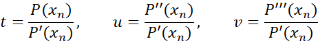
我们现在可以写出 Householder 的三阶方法如下

Householder 三阶的特征收敛阶效率指数为 4^(1/4)=1.41
Householder 三阶方法的效率指数为 1.41,与 Newton 和 Halley 方法一致。每次迭代,正确的数字位数都会翻四倍。
与 Newton 方法等效,重根的处理可以使用 Householder 三阶约化因子 3/(m+2) 来实现,通过将步长乘以反向因子,我们应该确保即使对于重根也能获得四次收敛速率。
我们修改后的 Householder 三阶方法将是

或者使用与之前相同的代入

从 Halley 迭代的演练中可以清楚地看出,我们可以保持相同的框架,只需替换迭代步骤即可。例如,去掉 Halley 步,换上 Householder 三阶方法。
高阶方法之间的比较
为了看看它在不同方法下的表现,让我们以一个简单的多项式为例。
P(x)= (x-2)(x+2)(x-3)(x+3)=x⁴-13x²+36
上述多项式对大多数方法来说都很简单。此外,正如您所看到的,高阶方法需要更少的迭代次数。然而,每次迭代需要做的工作也更多。
| 方法 | Newton | Halley | Householder 三阶 |
| 迭代 | 根 | 根 | 根 |
| 初始猜测 | 0.8320502943378436 | 0.8320502943378436 | 0.8320502943378436 |
| 1 | 2.2536991416170737 | 1.6933271400922734 | 2.033435992687734 |
| 2 | 1.9233571772166798 | 1.9899385955094577 | 1.9999990577501767 |
| 3 | 1.9973306906698116 | 1.9999993042509177 | 2 |
| 4 | 1.999996107736492 | 2 | |
| 5 | 1.9999999999916678 | ||
| 6 | 2 |
这是另一个例子。考虑有 6 个根在 1,2,3,4,5,6 的多项式。
P(x)=x⁶-21x⁵+175x⁴-735x³+1624x²-1764x+720
| 方法 | Newton | Halley | Householder 三阶 |
| 总迭代次数 | 21 | 16 | 14 |
| 比率 | 1 | 0.76 | 0.67 |
| 收敛阶 | 2 | 3 | 4 |
| 收敛比 | 1 | 0.67 | 0.5 |
列出的是每种方法的总迭代次数。理想情况下,Halley 应该只需要 Newton 方法所需迭代次数的 67% 就能完成工作。然而,它实际需要 76%。Householder 三阶方法也是如此,它理想情况下应该只需要 Newton 方法迭代次数的一半,但实际需要 67%。之所以不匹配,是因为收敛阶只在接近根时才适用。通常需要几次迭代才能接近根,而在这个过程中,会在复平面上游走,寻找到达根的路径。请参阅下面的各方法实测收敛阶的图像。当跟踪发生时,每种方法都遵循其收敛阶。


其他高阶方法
存在其他高阶方法,它们试图在多点方案中避免计算二阶和三阶导数。例如,Ostrowski 多点方法的效率指数为 1.59,是一种四阶方法。然而,您甚至可以找到其他方法,它们在不使用导数的情况下生成五阶、六阶、七阶甚至九阶的方法。缺点之一是,对于许多多点方法,没有修改版本能够有效地处理重根。
尽管存在重根的缺点,第六部分将介绍 Ostrowski 多点方法,并探讨我们如何仍然能够有效地处理重根。
在第四部分,我们将介绍 Laguerre 方法,在第五部分,我们将介绍一种同时迭代所有根的方法(Weierstrass 或 Durand-Kerner)。
建议
由于这些方法的效率指数相当,因此与 Newton 方法相比,使用 Halley 或 Householder 三阶方法没有任何优势。我建议坚持使用第一部分和第二部分介绍的 Newton 方法。
结论
我们已经构建了一个基于第一部分和第二部分建立的框架的改进型 Halley 方法,以高效且稳定地找到实系数多项式的根。虽然第一部分侧重于复系数多项式(其根仍可以是实数),但第二部分深入研究了实系数多项式。第三部分探讨了对 Halley 方法等高阶方法进行调整所需的修改,而第四部分将演示将 Laguerre 方法等替代方法集成到同一框架的简便性。一个展示这些不同方法的基于 Web 的多项式求解器可供进一步探索,可以在 http://www.hvks.com/Numerical/websolver.php 上找到,它演示了许多这些方法的效果。
参考文献
- H. Vestermark. A practical implementation of Polynomial root finders. Practical implementation of Polynomial root finders vs 7.docx (www.hvks.com)
- Madsen. A root-finding algorithm based on Newton Method, Bit 13 (1973) 71-75。
- A. Ostrowski, Solution of equations and systems of equations, Academic Press, 1966。
- Wikipedia Horner’s Method: https://en.wikipedia.org/wiki/Horner%27s_method
- Adams, D A stopping criterion for polynomial root finding. Communication of the ACM Volume 10/Number 10/ October 1967 Page 655-658
- Grant, J. A. & Hitchins, G D. Two algorithms for the solution of polynomial equations to limiting machine precision. The Computer Journal Volume 18 Number 3, pages 258-264
- Wilkinson, J H, Algebraic Processes中的舍入误差, Prentice-Hall Inc, Englewood Cliffs, NJ 1963
- McNamee, J.M., Numerical Methods for Roots of Polynomials, Part I & II, Elsevier, Kidlington, Oxford 2009
- H. Vestermark, “A Modified Newton and higher orders Iteration for multiple roots.”, www.hvks.com/Numerical/papers.html
- M.A. Jenkins & J.F. Traub, ”A three-stage Algorithm for Real Polynomials using Quadratic iteration”, SIAM J Numerical Analysis, Vol. 7, No.4, December 1970。
历史
- 2023 年 11 月 10 日:初稿