快速稳定的多项式求根器 - 第六部分

目录

• 引言
• 为什么选择 Ostrowski 方法？
• Ostrowski 的多点法
• 如何处理重根
• Ostrowski 方法与其他经典方法相比如何？
• 修改什么？
• Ostrowski 多点法的实现
• C++ 代码
• 示例 1
• 示例 2
• 示例 3
• 建议
• 最后的 remarks
• 参考文献
• 历史

引言

这是关于各种求根方法系列的第六篇也是最后一篇文章。我们将介绍所谓的“多点法”，我相信它最早是由 Ostrowski 在六十年代发明的。顾名思义，您会进行一系列中间点步骤，旨在降低计算需求，但同时保持比传统方法更高的收敛速度。Ostrowski 的成就是开发了一种四阶收敛速率，但只需要评估多项式 P(x) 及其一阶导数 P'(x)。即使我们需要采取额外的中间步骤，我们仍然可以保持系列文章第一至第四部分中建立的框架。

为什么选择 Ostrowski 方法？

Alexander Ostrowski (1893–1986) 是一位数学家，他在数值分析、数论和代数等多个领域做出了杰出贡献。Ostrowski 出生于当时俄国帝国的一部分基辅，拥有跨越多个国家和机构的多元化且广泛的学术生涯。

Alexander Ostrowski 在数值分析领域做出了杰出贡献，尤其是在开发寻找多项式根的方法方面。他最著名的贡献之一与多项式求根的多点法有关。这些方法是对牛顿法等经典迭代方法的扩展，它们旨在通过同时使用多个点或迭代来提高收敛速度和精度。

Ostrowski 在该领域的工作是为高效查找多项式根而设计的更广泛的数值算法的一部分，这是数值数学中的一个基本问题。他的研究对开发当今计算数学中使用的高级算法和技术产生了影响。

Ostrowski 贡献了两种不同的多项式求根方法。一种是本文介绍的多点法，另一种是平方根法。平方根法使用迭代

其中 m 是当重数 m > 1 时的修正。
然而，在本文中，我们将介绍多点公式

Ostrowski 的多点法引发了研究热潮，其他作者提出了具有 4-9 收敛速率的方法。作为这种极端研究的一个例子，Kumar 提供了下面的 9 阶方法。

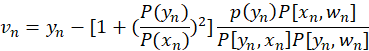
其中 P{x_n,w_n]=

请注意，对于 Kumar 方法，无需评估 P(x) 的任何导数。

Ostrowski 的多点法

Ostrowski 的多点法是

此方法之所以引人注目，是因为它实现了四阶收敛速率，并且只需要评估 P(x) 两次和一阶导数 P'(x)。这产生了 4^1/3=1.59 的效率指数，优于牛顿法和 Halley 法。第一步是标准的牛顿迭代，然后增强步长，产生四阶收敛。然而，当处理重根时，它与其他方法一样，收敛速度会下降到线性。

如何处理重根

好吧，一个解决方案是认识到第一步中间迭代是经典的牛顿迭代，它有一个可以有效处理重根的修改版本。添加修改后的牛顿迭代，您将获得一个处理重数 > 1 的方法；见下文。

阶段 1

阶段 2

然而，第二种改进对于 m > 1 的情况效果不佳。因此，我的方法是：

• 当迭代步 x_n 不接近根，并且我们看到使用多步和/或缩短步长（参见牛顿法的描述）有所改进时，则坚持使用这种修改后的牛顿方法。
• 首先，当您没有看到使用多步检查和/或步长缩短的任何改进时，则执行第二种改进，并为剩余的迭代获得四阶收敛。那么，重数大于一怎么办？这不成问题，因为它将使牛顿法保持在第一阶段，并二次收敛到该根，在这种特殊情况下，Ostrowski 的多点法将不是四阶方法，但对于简单根，它将是四阶方法。

Ostrowski 方法与其他经典方法相比如何？

为了了解它如何与不同的方法协同工作，让我们来看一下针对简单多项式的方法。

P(x)= (x-2)(x+2)(x-3)(x+3)=x^4-13x^2+36

上述多项式对大多数方法来说都很容易。此外，正如您所见，高阶方法需要更少的迭代次数。然而，每次迭代也需要做更多的工作。

方法	Newton	Halley	Household 3rd	Ostrowski
迭代	x	x	x	x
起始猜测	0.8320502943378436	0.8320502943378436	0.8320502943378436	0.8320502943378436
1	2.2536991416170737	1.6933271400922734	2.033435992687734	2.0863365344560694
2	1.9233571772166798	1.9899385955094577	1.9999990577501767	1.999968127551831
3	1.9973306906698116	1.9999993042509177	2	2
4	1.999996107736492	2
5	1.9999999999916678
6	2

这是以下示例：

第一个根最终是一个复共轭根 x=(1-i)，第三个根是另一个复共轭根，位于 (+2-i)，最后一个根直接找到为 x=5。请注意，搜索总是从实轴开始，然后在几次迭代后旋转到复平面。

上图显示了 Ostrowski 方法在逼近根时的收敛速度约为 4，符合预期。

修改什么？

与牛顿法（第二部分）相比，我们可以很幸运地重用牛顿法中已有的代码。

第二部分中的步骤包括：

1. 寻找一个初始点
2. 执行 Ostrowski 多点迭代，包括通过 Horner 方法进行多项式求值
3. 计算最终上限
4. 多项式降阶
5. 求解二次方程

Ad 1,3,4,5）将与牛顿法相同，无需修改

Ad 2）我们可以在计算最终上限后简单地将以下代码添加到 Stage 2 代码中，以实现 Ostrowski 多点法。

// Perform the Ostrowski multi-point step
// Pz is P(yn), pzprev is P(zn)
// Do the Ostrowski step as the second part of the multi-point iteration
z = z - pzprev.pz / (pzprev.pz - complex<double>(2) * pz.pz) * pz.pz / p1z.pz;
pz = horner(coeff, z); // Evaluate the new iteration point

Ostrowski 多点法的实现

这是与第二部分和第三部分相同的源，除了需要评估 Ostrowski 多点迭代步骤而不是牛顿法或 Halley 法的更改。

这个求根器的实现遵循第一部分中的方法布局。

1. 首先，我们消除零根（等于零的根）
2. 然后，我们找到一个合适的起点来开始我们的牛顿迭代，这还包括基于 P(x) 可接受值的初步终止条件，我们将停止当前迭代。
3. 开始 Ostrowski 迭代
   1. 第一步是找到 dx_n=P(x_n)/P’(x_n)，当然，要决定当 P’(x_n) 为零时该怎么办。当这种情况发生时，通常是由于局部最小值，最好的办法是通过因子 dx_n=dx_n(0.6+i0.8)m 来改变方向。这相当于将方向旋转 53 度（奇数次）并乘以因子 m。在这种情况下，m = 5 是一个合理的值。
   2. 此外，很容易意识到如果 P’(x_n)~0。您可能会得到一个不合理的步长 dx_n，因此引入一个限制因子，如果 abs(dx_n)>5·abs(dx_n-1) 则减小当前步长，使其小于前一次迭代的步长。同样，您通过 dx_n=dx_n(0.6+i0.8)5(abs(dx_n-1)/abs(dx_n)) 来改变方向。
   3. 以上两项修改使得该方法非常稳健，并且总是收敛到根。
   4. 下一个问题是处理重数 > 1 的问题，这会将二阶收敛速度降低到线性收敛速度。在找到合适的 dx_n 并得到新的 后，我们查看 P(x_n+1)>P(x_n)：如果是，我们查看修正后的 x_n+1=x_n-0.5dx_n，如果 P(x_n+1)≥P(x_n) 则我们使用原始的 x_n+1 作为下一次迭代的新起点。如果不是，那么我们接受 x_n+1 作为一个更好的选择，并继续寻找新修正的 x_n+1=x_n-0.25dx_n。另一方面，如果新的 P(x_n+1)≥P(x_n)，我们使用前一个 x_n+1 作为下一次迭代的新起点。如果不是，那么我们假设我们正在接近一个新的鞍点，并且方向通过 dx_n=dx_n(0.6+i0.8) 改变，我们使用 x_n+1=x_n-dx_n 作为下一次迭代的新起点。
      另一方面，如果 P(x_n+1)≤P(x_n )：那么我们正在朝着正确的方向前进，然后我们继续朝着这个方向前进，使用 x_n+1=x_n-mdx_n, m=2,..,n，只要 P(x_n+1)≤P(x_n )，并使用最佳的 m 进行下一次迭代。这个过程的好处是，如果存在重数为 m 的根，那么 m 也是步长大小的最佳选择，这将即使对于重根也能保持二阶收敛速率。最后两个步骤与牛顿法相同。
   5. 当进入收敛圆（第二阶段）时，我们跳过第四步，只需添加 Ostrowski 的第二步即可完成一次迭代。
4. 子过程 1 到 5 继续进行，直到达到停止条件，然后接受根 x_n 并将其降阶处理。使用降阶后的多项式启动新的根搜索。

我们将迭代分为两个阶段。第一阶段和第二阶段。在第一阶段，我们试图进入收敛圆，在那里我们确信 Ostrowski 方法将收敛到一个根。由于第一步是标准的牛顿迭代，我们将使用与牛顿法相同的计算。当我们进入该圆时，我们将自动切换到第二阶段。在第二阶段，我们跳过子步骤 4，只使用未经修改的牛顿迭代： 然后是 Ostrowski 的第二步： 直到满足停止条件。如果我们离开了收敛圆，我们将切换回第一阶段并继续迭代。
我们使用与牛顿法和 Halley 法相同的标准来切换到第二阶段。

现在我们拥有确定何时切换到阶段 2 所需的所有信息。

C++ 代码

下面的 C++ 代码使用 Ostrowski 的方法找到具有实系数多项式的多项式根。为了实现 Ostrowski 的方法，与牛顿版本相比，只做了很少的改动。我们只添加了以下几行代码。

// Perform the Ostrowski multi-point step
// Pz is P(yn), pzprev is P(zn)
// Do the Ostrowski step as the second part of the multi-point iteration
z = z - pzprev.pz / (pzprev.pz - complex<double>(2) * pz.pz) * pz.pz / p1z.pz;
pz = horner(coeff, z); // Evaluate the new iteration point

切换到第二阶段时。

Below is the full source.
/*
 *******************************************************************************
 *
 *                       Copyright (c) 2023
 *                       Henrik Vestermark
 *                       Denmark, USA
 *
 *                       All Rights Reserved
 *
 *   This source file is subject to the terms and conditions of
 *   Henrik Vestermark Software License Agreement which restricts the manner
 *   in which it may be used.
 *
 *******************************************************************************
*/

/*
 *******************************************************************************
 *
 * Module name     :   Ostrowski.cpp
 * Module ID Nbr   :
 * Description     :   Solve n degree polynomial using Ostrowski multi-point method
 * --------------------------------------------------------------------------
 * Change Record   :
 *
 * Version    Author/Date        Description of changes
 * -------  -------------    ----------------------
 * 01.01    HVE/24Dec2023    Initial release
 *
 * End of Change Record
 * --------------------------------------------------------------------------
*/

// define version string 
static char _VOSTROWSKI_[] = "@(#)testOstrowski.cpp 01.01 -- Copyright (C) Henrik Vestermark";

#include <algorithm>
#include <vector>
#include <complex>
#include <iostream>
#include <functional>

using namespace std;

constexpr int       MAX_ITER = 50;

// Find all polynomial zeros using a modified Newton method
// 1) Eliminate all simple roots (roots equal to zero)
// 2) Find a suitable starting point
// 3) Find a root using Newton
// 4) Divide the root up in the polynomial reducing its order with one
// 5) Repeat steps 2 to 4 until the polynomial is of the order of two 
//    whereafter the remaining one or two roots are found by the direct formula
// Notice:
//      The coefficients for p(x) is stored in descending order. 
//      coefficients[0] is a(n)x^n, coefficients[1] is a(n-1)x^(n-1),...,  
//      coefficients[n-1] is a(1)x, coefficients[n] is a(0)
//
static vector<complex<double>> PolynomialRootsOstrowski(const vector<double>& coefficients)
{
    struct eval { complex<double> z{}; complex<double> pz{}; double apz{}; };
    const complex<double> complexzero(0.0);  // Complex zero (0+i0)
    size_t n;       // Size of Polynomial p(x)  
    eval pz;        // P(z)
    eval pzprev;    // P(zprev)
    eval p1z;       // P'(z)
    eval p1zprev;   // P'(zprev)
    complex<double> z;      // Use as temporary variable
    complex<double> dz;     // The current stepsize dz
    int itercnt;    // Hold the number of iterations per root
    vector<complex<double>> roots;  // Holds the roots of the Polynomial
    vector<double> coeff(coefficients.size()); // Holds the current coefficients of P(z)

    copy(coefficients.begin(), coefficients.end(), coeff.begin());
    // Step 1 eliminate all simple roots
    for (n = coeff.size() - 1; n > 0 && coeff.back() == 0.0; --n)
        roots.push_back(complexzero);  // Store zero as the root

    // Compute the next starting point based on the polynomial coefficients
    // A root will always be outside the circle from the origin and radius min
    auto startpoint = [&](const vector<double>& a)
    {
        const size_t n = a.size() - 1;
        double a0 = log(abs(a.back()));
        double min = exp((a0 - log(abs(a.front()))) / static_cast<double>(n));

        for (size_t i = 1; i < n; i++)
            if (a[i] != 0.0)
            {
                double tmp = exp((a0 - log(abs(a[i]))) / static_cast<double>(n - i));
                if (tmp < min)
                    min = tmp;
            }

        return min * 0.5;
    };

    // Evaluate a polynomial with real coefficients a[] at a complex point z and
    // return the result 
    // This is Horner's methods avoiding complex arithmetic
    auto horner = [](const vector<double>& a, const complex<double> z)
    {
        const size_t n = a.size() - 1;
        double p = -2.0 * z.real();
        double q = norm(z);
        double s = 0.0;
        double r = a[0];
        eval e;

        for (size_t i = 1; i < n; i++)
        {
            double t = a[i] - p * r - q * s;
            s = r;
            r = t;
        }

        e.z = z;
        e.pz = complex<double>(a[n] + z.real() * r - q * s, z.imag() * r);
        e.apz = abs(e.pz);
        return e;
    };

    // Calculate an upper bound for the rounding errors performed in a
    // polynomial with real coefficient a[] at a complex point z. 
    // (Adam's test)
    auto upperbound = [](const vector<double>& a, const complex<double> z)
    {
        const size_t n = a.size() - 1;
        double p = -2.0 * z.real();
        double q = norm(z);
        double u = sqrt(q);
        double s = 0.0;
        double r = a[0];
        double e = fabs(r) * (3.5 / 4.5);
        double t;

        for (size_t i = 1; i < n; i++)
        {
            t = a[i] - p * r - q * s;
            s = r;
            r = t;
            e = u * e + fabs(t);
        }
        t = a[n] + z.real() * r - q * s;
        e = u * e + fabs(t);
        e = (4.5 * e - 3.5 * (fabs(t) + fabs(r) * u) +
            fabs(z.real()) * fabs(r)) * 0.5 * pow((double)_DBL_RADIX, -DBL_MANT_DIG + 1);

        return e;
    };

   // Do Ostrowski iteration for polynomial order higher than 2
    for (; n > 2; --n)
    {
        const double Max_stepsize = 5.0; // Allow the next step size to be up to 
                                         // 5 times larger than the previous step size
        const complex<double> rotation = complex<double>(0.6, 0.8);  // Rotation amount
        double r;               // Current radius
        double rprev;           // Previous radius
        double eps;             // The iteration termination value
        bool stage1 = true;     // By default it start the iteration in stage1
        int steps = 1;          // Multisteps if > 1
        vector<double> coeffprime;

        // Calculate coefficients of p'(x)
        for (int i = 0; i < n; i++)
            coeffprime.push_back(coeff[i] * double(n - i));

        // Step 2 find a suitable starting point z
        rprev = startpoint(coeff);      // Computed startpoint
        z = coeff[n - 1] == 0.0 ? complex<double>(1.0) : complex<double>
                            (-coeff[n] / coeff[n - 1]);
        z *= complex<double>(rprev) / abs(z);

        // Setup the iteration
        // Current P(z)
        pz = horner(coeff, z);

        // pzprev which is the previous z or P(0)
        pzprev.z = complex<double>(0);
        pzprev.pz = coeff[n];
        pzprev.apz = abs(pzprev.pz);

        // p1zprev P'(0) is the P'(0)
        p1zprev.z = pzprev.z;
        p1zprev.pz = coeff[n - 1];       // P'(0)
        p1zprev.apz = abs(p1zprev.pz);

        // Set previous dz and calculate the radius of operations.
        dz = pz.z;                 // dz=z-zprev=z since zprev==0
        r = rprev *= Max_stepsize; // Make a reasonable radius of the 
                                   // maximum step size allowed
        // Preliminary eps computed at point P(0) by a crude estimation
        eps = 2 * n * pzprev.apz * pow((double)_DBL_RADIX, -DBL_MANT_DIG);

        // Start iteration and stop if z doesnt change or apz <= eps
        // we do z+dz!=z instead of dz!=0. if dz does not change z 
        // then we accept z as a root
        for (itercnt = 0; pz.z + dz != pz.z && pz.apz > eps && 
                                 itercnt < MAX_ITER; itercnt++)
        {
     // Calculate current P'(z)
            p1z = horner(coeffprime, pz.z);
            if (p1z.apz == 0.0)                 // P'(z)==0 then rotate and try again
                dz *= rotation * complex<double>(Max_stepsize);  // Multiply with 5 
                                                // to get away from saddlepoint
            else
            {
                dz = pz.pz / p1z.pz;  // next dz
                // Check the Magnitude of Newton's step
                r = abs(dz);
                if (r > rprev) // Large than 5 times the previous step size
                {   // then rotate and adjust step size to prevent 
                    // wild step size near P'(z) close to zero
                    dz *= rotation * complex<double>(rprev / r);
                    r = abs(dz);
                }
                rprev = r * Max_stepsize;  // Save 5 times the current step size for the 
                                           // next iteration check of reasonable step size
                // Calculate if stage1 is true or false. Stage1 is false if the 
                // Newton converge otherwise true
                z = (p1zprev.pz - p1z.pz) / (pzprev.z - pz.z);
                stage1 = (abs(z) / p1z.apz > p1z.apz / pz.apz / 4) || (steps != 1);
            }
            // Step accepted. Save pz in pzprev
            pzprev = pz;

            z = pzprev.z - dz;      // Next z
            pz = horner(coeff, z);  //ff = pz.apz;
            // Add this point all we have done is perform a Newton Step
            steps = 1;
            if (stage1)
            {  // Try multiple steps or shorten steps depending if P(z) 
               // is an improvement or not P(z)<P(zprev)
                bool div2;
                complex<double> zn;
                eval npz;

                zn = pz.z;
                for (div2 = pz.apz > pzprev.apz; steps <= n; ++steps)
                {
                    if (div2 == true)
                    {  // Shorten steps
                        dz *= complex<double>(0.5);
                        zn = pzprev.z - dz;
                    }
                    else
                        zn -= dz;  // try another step in the same direction

                    // Evaluate new try step
                    npz = horner(coeff, zn);
                    if (npz.apz >= pz.apz)
                        break; // Break if no improvement

                    // Improved => accept step and try another round of step
                    pz = npz;

                    if (div2 == true && steps == 2)
                    {   // To many shorten steps => try another direction and break
                        dz *= rotation;
                        z = pzprev.z - dz;
                        pz = horner(coeff, z);
                        break;
                    }
                }
            }
            else
            {   // calculate the upper bound of error using Adam's test 
                // for real coefficients
                // Now that we are within the convergence circle.
                eps = upperbound(coeff, pz.z);
                // Perform the Ostrowski multi-point step
                // Pz is P(yn), pzprev is P(zn)
                // Do the Ostrowski step as the second part of the multi-point iteration
                z = z - pzprev.pz / 
                        (pzprev.pz - complex<double>(2) * pz.pz) * pz.pz / p1z.pz;
                pz = horner(coeff, z); // Evaluate the new iteration point
            }
        }

        // Real root forward deflation.
        //
        auto realdeflation = [&](vector<double>& a, const double x)
        {
            const size_t n = a.size() - 1;
            double r = 0.0;

            for (size_t i = 0; i < n; i++)
                a[i] = r = r * x + a[i];

            a.resize(n);    // Remove the highest degree coefficients.
        };

        // Complex root forward deflation for real coefficients
        //
        auto complexdeflation = [&](vector<double>& a, const complex<double> z)
        {
            const size_t n = a.size() - 1;
            double r = -2.0 * z.real();
            double u = norm(z);

            a[1] -= r * a[0];
            for (int i = 2; i < n - 1; i++)
                a[i] = a[i] - r * a[i - 1] - u * a[i - 2];

            a.resize(n - 1); // Remove top 2 highest degree coefficients
        };

        // Check if there is a very small residue in the imaginary part by trying
        // to evaluate P(z.real). if that is less than P(z). 
        // We take that z.real() is a better root than z.
        z = complex<double>(pz.z.real(), 0.0);
        pzprev = horner(coeff, z);
        if (pzprev.apz <= pz.apz)
        { // real root 
            pz = pzprev;
            // Save the root
            roots.push_back(pz.z);
            realdeflation(coeff, pz.z.real());
        }
        else
        {   // Complex root
            // Save the root
            roots.push_back(pz.z);
            roots.push_back(conj(pz.z));
            complexdeflation(coeff, pz.z);
            --n;
        }

    }   // End Iteration

    // Solve any remaining linear or quadratic polynomial
    // For Polynomial with real coefficients a[], 
    // The complex solutions are stored in the back of the roots
    auto quadratic = [&](const std::vector<double>& a)
    {
        const size_t n = a.size() - 1;
        complex<double> v;
        double r;

        // Notice that a[0] is !=0 since roots=zero has already been handle
        if (n == 1)
            roots.push_back(complex<double>(-a[1] / a[0], 0));
        else
        {
            if (a[1] == 0.0)
            {
                r = -a[2] / a[0];
                if (r < 0)
                {
                    r = sqrt(-r);
                    v = complex<double>(0, r);
                    roots.push_back(v);
                    roots.push_back(conj(v));
                }
                else
                {
                    r = sqrt(r);
                    roots.push_back(complex<double>(r));
                    roots.push_back(complex<double>(-r));
                }
            }
            else
            {
                r = 1.0 - 4.0 * a[0] * a[2] / (a[1] * a[1]);
                if (r < 0)
                {
                    v = complex<double>(-a[1] / (2.0 * a[0]), 
                                         a[1] * sqrt(-r) / (2.0 * a[0]));
                    roots.push_back(v);
                    roots.push_back(conj(v));
                }
                else
                {
                    v = complex<double>((-1.0 - sqrt(r)) * a[1] / (2.0 * a[0]));
                    roots.push_back(v);
                    v = complex<double>(a[2] / (a[0] * v.real()));
                    roots.push_back(v);
                }
            }
        }
        return;
    };

    if (n > 0)
        quadratic(coeff);

    return roots;
}

示例 1

以下是上述源代码工作方式的示例。

For the real Polynomial:
+1x^4-10x^3+35x^2-50x+24
Start Ostrowski Iteration for Polynomial=+1x^4-10x^3+35x^2-50x+24
Stage 1=>Stop Condition. |f(z)|<2.13e-14
Start: z[1]=0.2 dz=2.40e-1 |f(z)|=1.4e+1
Iteration: 1
Ostrowski Step: z[1]=0.6 dz=-3.98e-1 |f(z)|=3.9e+0
Function value decrease=>try multiple steps in that direction
Try Step: z[1]=1 dz=-3.98e-1 |f(z)|=2.0e-1
: Improved. Continue stepping
Try Step: z[1]=1 dz=-3.98e-1 |f(z)|=9.9e-1
: No improvement. Discard the last try step
Iteration: 2
Ostrowski Step: z[1]=1 dz=3.87e-2 |f(z)|=1.6e-2
Function value decrease=>try multiple steps in that direction
Try Step: z[1]=1 dz=3.87e-2 |f(z)|=2.7e-1
: No improvement. Discard the last try step
Ostrowski Stage 2 Step: z[1]=1 dz=-2.63e-3 |f(z)|=5.3e-5
Iteration: 3
Ostrowski Step: z[1]=1 dz=-8.78e-6 |f(z)|=8.5e-10
In Stage 2. New Stop Condition: |f(z)|<2.18e-14
Ostrowski Stage 2 Step: z[1]=1 dz=-1.41e-10 |f(z)|=0
Stop Criteria satisfied after 3 Iterations
Final Ostrowski z[1]=1 dz=-8.78e-6 |f(z)|=0
Alteration=0% Stage 1=67% Stage 2=33%
Deflate the real root z=1
Start Ostrowski Iteration for Polynomial=+1x^3-9x^2+26x-24
Stage 1=>Stop Condition. |f(z)|<1.60e-14
Start : z[1]=0.5 dz=4.62e-1 |f(z)|=1.4e+1
Iteration: 1
Ostrowski Step: z[1]=1 dz=-7.54e-1 |f(z)|=3.9e+0
Function value decrease=>try multiple steps in that direction
Try Step: z[1]=2 dz=-7.54e-1 |f(z)|=6.4e-2
: Improved. Continue stepping
Try Step: z[1]=3 dz=-7.54e-1 |f(z)|=2.6e-1
: No improvement. Discard the last try step
Iteration: 2
Ostrowski Step: z[1]=2 dz=-2.95e-2 |f(z)|=2.7e-3
Function value decrease=>try multiple steps in that direction
Try Step: z[1]=2 dz=-2.95e-2 |f(z)|=5.4e-2
: No improvement. Discard the last try step
Ostrowski Stage 2 Step: z[1]=2 dz=-1.32e-3 |f(z)|=4.1e-6
Iteration: 3
Ostrowski Step: z[1]=2 dz=-2.06e-6 |f(z)|=1.3e-11
In Stage 2. New Stop Condition: |f(z)|<1.42e-14
Ostrowski Stage 2 Step: z[1]=2 dz=-6.36e-12 |f(z)|=0
Stop Criteria satisfied after 3 Iterations
Final Ostrowski z[1]=2 dz=-2.06e-6 |f(z)|=0
Alteration=0% Stage 1=67% Stage 2=33%
Deflate the real root z=2.0000000000000004
Solve Polynomial=+1x^2-7x+11.999999999999996 directly
Using the Ostrowski Method, the Solutions are:
X1=1
X2=2.0000000000000004
X3=4.000000000000003
X4=2.9999999999999973
Time used: 0 msec. Solvable level: Easy

示例 2

同一个例子，只是有一个双根 x=1。我们看到每一步都是双步，与第一个根的重数为 2 相符。

For the real Polynomial:
+1x^4-9x^3+27x^2-31x+12
Start Ostrowski Iteration for Polynomial=+1x^4-9x^3+27x^2-31x+12
Stage 1=>Stop Condition. |f(z)|<1.07e-14
Start : z[1]=0.2 dz=1.94e-1 |f(z)|=6.9e+0
Iteration: 1
Ostrowski Step: z[1]=0.5 dz=-3.23e-1 |f(z)|=2.0e+0
Function value decrease=>try multiple steps in that direction
Try Step: z[1]=0.8 dz=-3.23e-1 |f(z)|=1.8e-1
: Improved. Continue stepping
Try Step: z[1]=1 dz=-3.23e-1 |f(z)|=1.4e-1
: Improved. Continue stepping
Try Step: z[1]=1 dz=-3.23e-1 |f(z)|=8.9e-1
: No improvement. Discard the last try step
Iteration: 2
Ostrowski Step: z[1]=1 dz=8.71e-2 |f(z)|=3.1e-2
Function value decrease=>try multiple steps in that direction
Try Step: z[1]=1 dz=8.71e-2 |f(z)|=9.6e-4
: Improved. Continue stepping
Try Step: z[1]=0.9 dz=8.71e-2 |f(z)|=6.5e-2
: No improvement. Discard the last try step
Iteration: 3
Ostrowski Step: z[1]=1 dz=-6.27e-3 |f(z)|=2.4e-4
Function value decrease=>try multiple steps in that direction
Try Step: z[1]=1 dz=-6.27e-3 |f(z)|=2.6e-8
: Improved. Continue stepping
Try Step: z[1]=1 dz=-6.27e-3 |f(z)|=2.3e-4
: No improvement. Discard the last try step
Iteration: 4
Ostrowski Step: z[1]=1 dz=-3.28e-5 |f(z)|=6.5e-9
Function value decrease=>try multiple steps in that direction
Try Step: z[1]=1 dz=-3.28e-5 |f(z)|=0
: Improved. Continue stepping
Try Step: z[1]=1 dz=-3.28e-5 |f(z)|=6.5e-9
: No improvement. Discard the last try step
Stop Criteria satisfied after 4 Iterations
Final Ostrowski z[1]=1 dz=-3.28e-5 |f(z)|=0
Alteration=0% Stage 1=100% Stage 2=0%
Deflate the real root z=0.9999999982094424
Start Ostrowski Iteration for Polynomial=+1x^3-8.000000001790557x^2+19.000000012533903x-12.000000021486692
Stage 1=>Stop Condition. |f(z)|<7.99e-15
Start : z[1]=0.3 dz=3.16e-1 |f(z)|=6.8e+0
Iteration: 1
Ostrowski Step: z[1]=0.8 dz=-4.75e-1 |f(z)|=1.5e+0
Function value decrease=>try multiple steps in that direction
Try Step: z[1]=1 dz=-4.75e-1 |f(z)|=1.3e+0
: Improved. Continue stepping
Try Step: z[1]=2 dz=-4.75e-1 |f(z)|=2.1e+0
: No improvement. Discard the last try step
Iteration: 2
Ostrowski Step: z[1]=0.9 dz=3.54e-1 |f(z)|=5.7e-1
Function value decrease=>try multiple steps in that direction
Try Step: z[1]=0.6 dz=3.54e-1 |f(z)|=3.7e+0
: No improvement. Discard the last try step
Ostrowski Stage 2 Step: z[1]=1 dz=-8.44e-2 |f(z)|=2.6e-2
Iteration: 3
Ostrowski Step: z[1]=1 dz=-4.35e-3 |f(z)|=9.5e-5
In Stage 2. New Stop Condition: |f(z)|<6.66e-15
Ostrowski Stage 2 Step: z[1]=1 dz=-1.58e-5 |f(z)|=9.5e-10
Iteration: 4
Ostrowski Step: z[1]=1 dz=-1.58e-10 |f(z)|=8.9e-16
In Stage 2. New Stop Condition: |f(z)|<6.66e-15
Ostrowski Stage 2 Step: z[1]=1 dz=1.48e-16 |f(z)|=8.9e-16
Stop Criteria satisfied after 4 Iterations
Final Ostrowski z[1]=1 dz=-1.58e-10 |f(z)|=8.9e-16
Alteration=0% Stage 1=50% Stage 2=50%
Deflate the real root z=1.0000000017905575
Solve Polynomial=+1x^2-7x+12 directly
Using the Ostrowski Method, the Solutions are:
X1=0.9999999982094424
X2=1.0000000017905575
X3=4
X4=3
Time used: 1 msec. Solvable level: Easy

示例 3

一个同时具有实根和复共轭根的测试多项式。

For the real Polynomial:
+1x^4-8x^3-17x^2-26x-40
Start Ostrowski Iteration for Polynomial=+1x^4-8x^3-17x^2-26x-40
Stage 1=>Stop Condition. |f(z)|<3.55e-14
Start : z[1]=-0.8 dz=-7.67e-1 |f(z)|=2.6e+1
Iteration: 1
Ostrowski Step: z[1]=-2 dz=1.65e+0 |f(z)|=7.0e+1
Function value increase=>try shorten the step
Try Step: z[1]=-2 dz=8.24e-1 |f(z)|=3.1e+0
: Improved=>Continue stepping
Try Step: z[1]=-1 dz=4.12e-1 |f(z)|=1.8e+1
: No improvement=>Discard last try step
Iteration: 2
Ostrowski Step: z[1]=-2 dz=6.27e-2 |f(z)|=1.5e-1
Function value decrease=>try multiple steps in that direction
Try Step: z[1]=-2 dz=6.27e-2 |f(z)|=3.7e+0
: No improvement. Discard the last try step
Ostrowski Stage 2 Step: z[1]=-2 dz=-2.74e-3 |f(z)|=1.4e-4
Iteration: 3
Ostrowski Step: z[1]=-2 dz=-2.58e-6 |f(z)|=2.6e-10
In Stage 2. New Stop Condition: |f(z)|<1.91e-14
Ostrowski Stage 2 Step: z[1]=-2 dz=-4.88e-12 |f(z)|=0
Stop Criteria satisfied after 3 Iterations
Final Ostrowski z[1]=-2 dz=-2.58e-6 |f(z)|=0
Alteration=0% Stage 1=67% Stage 2=33%
Deflate the real root z=-1.650629191439388
Start Ostrowski Iteration for Polynomial=+1x^3-9.650629191439387x^2-1.0703897408530487x-24.233183447530717
Stage 1=>Stop Condition. |f(z)|<1.61e-14
Start : z[1]=-0.8 dz=-7.92e-1 |f(z)|=3.0e+1
Iteration: 1
Ostrowski Step: z[1]=1 dz=-1.86e+0 |f(z)|=3.5e+1
Function value increase=>try shorten the step
Try Step: z[1]=0.1 dz=-9.30e-1 |f(z)|=2.5e+1
: Improved=>Continue stepping
Try Step: z[1]=-0.3 dz=-4.65e-1 |f(z)|=2.5e+1
: No improvement=>Discard last try step
Iteration: 2
Ostrowski Step: z[1]=-7 dz=6.71e+0 |f(z)|=7.2e+2
Function value increase=>try shorten the step
Try Step: z[1]=-3 dz=3.35e+0 |f(z)|=1.5e+2
: Improved=>Continue stepping
Try Step: z[1]=-2 dz=1.68e+0 |f(z)|=4.9e+1
: Improved=>Continue stepping
: Probably local saddlepoint=>Alter Direction: z[1]=(-0.4-i0.7) dz=(5.03e-1+i6.71e-1) |f(z)|=2.1e+1
Iteration: 3
Ostrowski Step: z[1]=(0.3-i2) dz=(-6.86e-1+i1.17e+0) |f(z)|=1.9e+1
Function value decrease=>try multiple steps in that direction
Try Step: z[1]=(1-i3) dz=(-6.86e-1+i1.17e+0) |f(z)|=8.4e+1
: No improvement. Discard the last try step
Ostrowski Stage 2 Step: z[1]=(-0.09-i2) dz=(4.13e-1-i3.17e-1) |f(z)|=2.6e+0
Iteration: 4
Ostrowski Step: z[2]=(-0.18-i1.5) dz=(8.33e-2+i2.00e-2) |f(z)|=8.1e-2
In Stage 2. New Stop Condition: |f(z)|<1.36e-14
Ostrowski Stage 2 Step: z[4]=(-0.1747-i1.547) dz=(-1.74e-3+i1.86e-3) |f(z)|=6.2e-5
Iteration: 5
Ostrowski Step: z[7]=(-0.1746854-i1.546869) dz=(1.94e-6-i4.50e-8) |f(z)|=4.2e-11
In Stage 2. New Stop Condition: |f(z)|<1.36e-14
Ostrowski Stage 2 Step: z[13]=(-0.1746854042803-i1.546868887231) dz=(-3.03e-13+i1.29e-12) |f(z)|=3.6e-15
Stop Criteria satisfied after 5 Iterations
Final Ostrowski z[7]=(-0.1746854-i1.546869) dz=(1.94e-6-i4.50e-8) |f(z)|=3.6e-15
Alteration=20% Stage 1=60% Stage 2=40%
Deflate the complex conjugated root z=(-0.17468540428030602-i1.546868887231396)
Solve Polynomial=+1x-10 directly
Using the Ostrowski Method, the Solutions are:
X1=-1.650629191439388
X2=(-0.17468540428030602-i1.546868887231396)
X3=(-0.17468540428030602+i1.546868887231396)
X4=10
Time used: 1 msec. Solvable level: Easy

迭代过程趋向于前两个根。

建议

由于效率指数高于牛顿法、Halley 法和其他方法，Ostrowski 的多点法值得考虑。但是，有一个众所周知的缺陷，即在遇到重根时收敛阶数会降低。由于在这种情况下仍能保持二阶收敛阶数，因此与牛顿法相比，由于其更高的效率指数 1.59（牛顿法为 1.41），在处理相距较远的根时，可以认为它更好。

最后的 remarks

在本系列文章中，我们介绍了许多经典方法，例如不动点法、多点法、并行方法等。然而，我遗漏了两种也值得一提的方法，那就是著名的 Jenkins-Traub “黑盒”方法，当然还有特征值方法。这两种方法都值得单独写一篇论文，也许可以作为本文系列的进一步扩展。尽管第六部分介绍了许多截然不同的方法，但它们都可以集成到第一部分和第二部分建立的同一个框架中，从一种方法切换到另一种方法，您只需要在这里或那里更改几行代码，同时仍然保持每种方法的稳健性、弹性和高效实现。

一个展示这些各种方法的基于 Web 的多项式求解器可供进一步探索，可以在 多项式根 (http://hvks.com/Numerical/websolver.php) 上找到，它演示了所有这些方法。

参考文献

1. H. Vestermark. A practical implementation of Polynomial root finders. Practical implementation of Polynomial root finders vs 7.docx (www.hvks.com)
2. Madsen. A root-finding algorithm based on Newton Method, Bit 13 (1973) 71-75。
3. A. Ostrowski, Solution of equations and systems of equations, Academic Press, 1966。
4. Wikipedia Horner’s Method: https://en.wikipedia.org/wiki/Horner%27s_method
5. Adams, D A stopping criterion for polynomial root finding. Communication of the ACM Volume 10/Number 10/ October 1967 Page 655-658
6. Grant, J. A. & Hitchins, G D. Two algorithms for the solution of polynomial equations to limiting machine precision. The Computer Journal Volume 18 Number 3, pages 258-264
7. Wilkinson, J H, Algebraic Processes中的舍入误差, Prentice-Hall Inc, Englewood Cliffs, NJ 1963
8. McNamee, J.M., Numerical Methods for Roots of Polynomials, Part I & II, Elsevier, Kidlington, Oxford 2009
9. H. Vestermark, “A Modified Newton and higher orders Iteration for multiple roots.”, www.hvks.com/Numerical/papers.html
10. M.A. Jenkins & J.F. Traub, ”A three-stage Algorithm for Real Polynomials using Quadratic iteration”, SIAM J Numerical Analysis, Vol. 7, No.4, December 1970。

历史

• 2024 年 1 月 8 日：原始提交的一些图像丢失
• 2024 年 1 月 6 日：Ostrowski 多点法的初始版本