
无监督学习 - 聚类和 K-Means
5.00/5 (2投票s)
- 1. 引言
- 2. 问题
- 3. 场景
- 4. 使用的符号和编码指南
- 5. 解决方案
- 6. 外部参考
- 7. 基数计数 'k' 的问题
- 8. 实验结果
- 9. 它是如何工作的?
- 10. 关于距离度量和测量的说明
- 11. 总结
- 12. 参考文献
- 13. 练习
- 14. K-Means 聚类进一步探讨
1. 引言
在已知标签的数据样本学习中,根据学习到的带标签数据来确定实验数据标签的数学公式/模型是监督学习模型。当数据样本的标签事先未知时,找到样本数据标签的一种解决方案是找到数据集中的各种簇(数据分组),然后在计算后期对簇进行标记。这种在模型中创建簇以便在计算后期标记样本(当数据集样本标签事先未知时)的方法,是无监督学习模型。涉及无标签样本数据簇形成的一种算法是 k-means 算法。
2. 问题
如何将样本数据集组装成不同的簇,使得每个样本数据(文档)只属于一个簇组。我们有一个训练集样本 {x(1),..., x(n)} 或 {d(1),…,d(n)},并希望将数据分组为几个内聚的“簇”。这里,x(i) ∈ Rd,但没有给出标签 y(i)。这是无监督学习问题。簇形成解决方案应由各种距离度量支持。
3. 场景
在一般场景下,无论地理分布还是逻辑分布的样本数据,都存在于“k”个簇中。每个簇围绕一个“质心/均值”形成,而一个特定簇中的所有数据样本(文档)都比其他簇的均值更接近其自身的簇“均值”(即欧几里得距离)。因此,每个簇的方差或惯性最小。整个数据集的总惯性/方差达到最低。

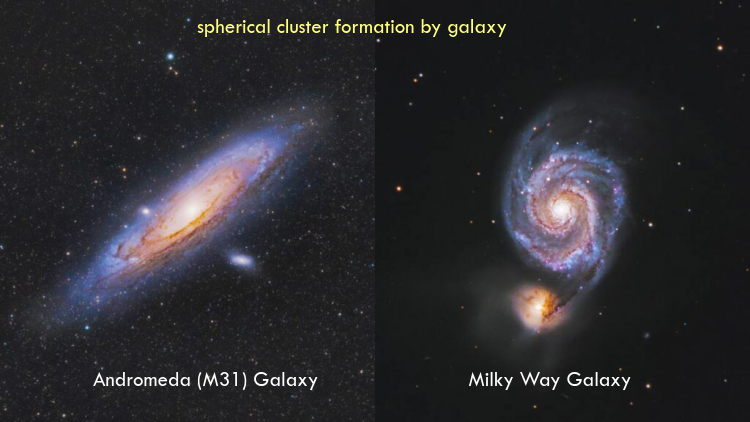
在空间领域,一颗恒星是许多空间天体的平均值,太阳平均簇被标记为太阳系。黑洞是围绕它形成星系的恒星簇的平均恒星。人马座 A 是银河系的黑洞平均值。簇在三维空间中是球形的。
4. 使用的符号和编码指南
4.1 使用的符号

注意:词语“质心和均值”、“样本数据和文档”可互换使用。
4.2 编码指南
- 识别外部和内部标识符。任何外部标识符,即函数参数或通过“from <module> import <name> as <name>”导入的名称,都写成 e_<identifier>。
- 列表变量以字母“s”结尾,即“document”是非序列(列表/元组),而“documents”是序列(列表/元组)。
   from modulea import classa as e_classa
   ....
   def func(e_par1, e_par2, e_samples, *e_args, *e_kwarg):
    #e_samples and e_args being sequences
    print('{(e_par1,e_par,e_samples,e_args,e_kwarg)=}')
5. 解决方案
找到数据集中存在的“k”个簇的一种可能的数学计算方法是 k-means 算法。该算法不改变数据集样本的位置,而是为每个簇引入新的独立质心/均值点。一组“k”个新的质心/均值点。
5.1 设计
一组“k”个随机种子均值/质心在开始时从数据集中确定(初始均值)。基于到所有“k”个均值的距离(例如欧几里得距离、余弦距离),每个样本数据/文档被重新分配到最近的均值。每个均值/质心的位置根据其自身簇中所有数据样本/文档的均值位置重新计算。这导致数据样本在重新分配阶段移动其均值,而均值在重新计算阶段移动其位置(在其自己的簇内)。无论是重新分配还是重新计算,都不会收敛,最终会形成簇。
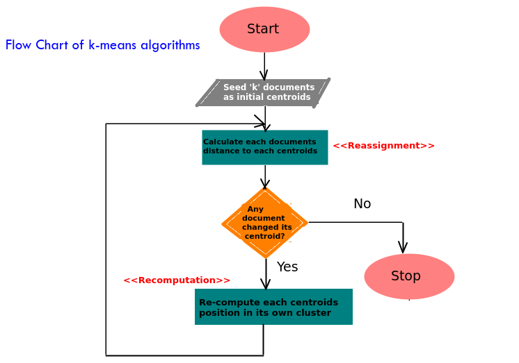
5.1.1 算法步骤
- 随机选择“k”个文档点作为初始均值。
- 每个样本数据找到最近的均值,通过某种数学距离公式(例如欧几里得或余弦距离)从“k”个均值中计算得出。这称为重新分配。
- 每个“k”个均值在其自身的簇内重新计算其位置,即与簇中所有文档的数学平均距离。这称为重新计算。
- 重复步骤 2 和 3,直到样本数据/文档停止转移到另一个簇。停止重新分配。

5.1.2 算法步骤可视化

5.1.3 算法流程图
算法的流程图可推导如下。
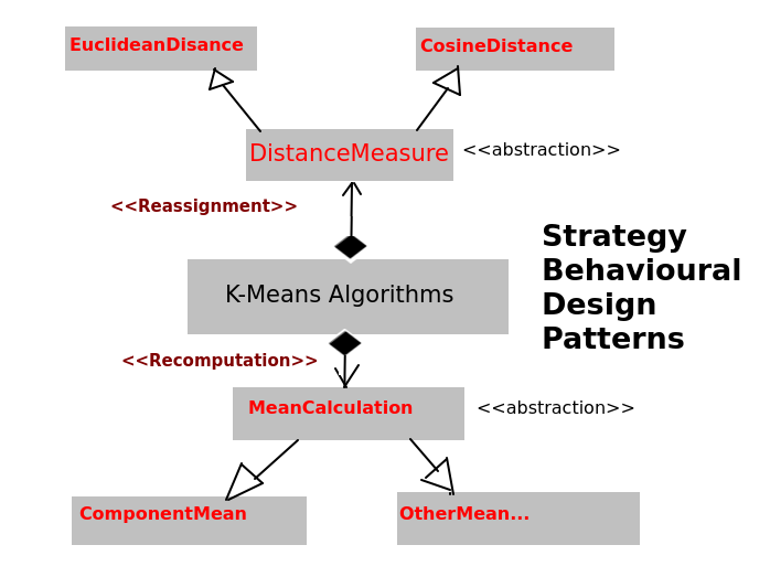
5.1.4 策略设计模式
它遵循策略行为设计模式。
5.2 算法
k-means 算法可以采用多种可能的距离度量(例如欧几里得/余弦距离)配方进行重新分配阶段,以及多种可能的均值计算度量(例如数学均值)配方进行重新计算阶段。
5.2.1 从零开始的算法
使用欧几里得距离度量和平均数学均值从零开始实现算法的 Python 代码。
import numpy as np,random
from sklearn.metrics.pairwise import euclidean_distances,cosine_distances
def kmeans(e_samples,e_initmeans):
 '''-> returns dict of labels and means'''
 print(f'kmeans {e_samples[:3]=} {e_initmeans=}')
 means=e_initmeans
 #initialize label against each sample as -1
 labels=[[-1]*len(e_samples),None]
 while True:
  #ReAssignment
  labels[1]=np.argmin(euclidean_distances(e_samples,means),axis=1).tolist()
  print(f'kmeans --ReAssignment-- {labels=}')
  if labels[0]==labels[1]:
   return dict(labels=labels[0],means=means)
  labels[0]=labels[1]
  #ReComputation
  means=[np.mean([e_samples[count] for count in range(len(e_samples)) if labels[0][count]==i],axis=0).tolist() for i in range(len(e_initmeans))]
  print(f'kmeans --ReComputation-- {means=}')
函数 `kmeans` 接收初始均值 `e_initmeans` 作为外部函数参数。`labels` 是 `labels[0]` 旧标签和 `labels[1]` 新标签。如果重新分配阶段给 `labels[1]`(与旧标签 `labels[0]` 不同)带来变化,则会计算均值(重新计算)。它使用辅助函数 `get_means` 和 `matplotlib_imaging` 分别计算初始均值和绘制 matplotlib 图形。它以字典形式返回标签(作为 `labels[0]`)和均值。
def get_means(*,e_samples,e_rand_state,e_k):
 print(f'get_means {e_samples[:10]=} {e_rand_state=} {e_k=}')
 return np.array(list(set(tuple(x) for x in e_samples)))[np.random.RandomState(e_rand_state).choice(len(set(tuple(x) for x in e_samples)),e_k,replace=False)].tolist()

from matplotlib import pyplot as plt
import re,os
def matplotlib_imaging(e_arg):
 color=('red','green','blue')
 fig,axes=plt.subplots()
 if e_arg:
  print(f'matplotlib_pyplot e_arg={dict({x:e_arg[x] if x!= "samples" else e_arg[x][:3] for x in e_arg})}')
  [axes.scatter(*zip(*[e_arg['samples'][count] for count in range(len(e_arg['samples'])) if e_arg['labels'][count]==i or e_arg['labels'][count]==-1]), s=10, label=str(i),c=[c] if e_arg['labels'][0]!=-1 else [[0,0,0]]) for i,c in enumerate(color[0:len(e_arg['means'])])]
  axes.scatter(*zip(*e_arg['means']), s=90, marker='*',c=color[0:len(e_arg['means'])])
  axes.legend()
  imagename="matplotlib_imaging_"+str(max([int(re.sub(r'^.*?(\d+)[.]png$',r'\1',i)) for i in os.listdir() if re.search(r'matplotlib_imaging_\d+[.]png',i,flags=re.I)] or [-1])+1)+".png"
  print(f'matplotlib_imaging saving to file {imagename}')
  fig.savefig(imagename)
`get_means()` 函数通过外部提供的 `e_rand_state` 函数参数,例如 `e_rand_state=[0,None]`,通过不同的 RandomState 初始种子随机计算初始均值。
运行 `rand_state=0` 和 `rand_state=None` 的代码。
输入
samples=[[-14,-5],[13,13],[20,23],[-19,-11],[-9,-16],[21,27],[-49,15],[26,13],[-46,5],[-34,-1],[11,15],[-49,0],[-22,-16],[19,28],[-12,-8],[-13,-19],[-41,8],[-11,-6],[-25,-9],[-18,-3]]
print(f'--- KMEANS FROM SCRATCH ---')
print(f'{"RANDOM STATE -> 0":-^40}')
matplotlib_imaging(dict(samples=samples,**kmeans(e_samples=samples,e_initmeans=get_means(e_samples=samples,e_rand_state=0,e_k=3))))
print(f'{"RANDOM STATE -> None":-^40}')
matplotlib_imaging(dict(samples=samples,**kmeans(e_samples=samples,e_initmeans=get_means(e_samples=samples,e_rand_state=None,e_k=3))))
输出
--- KMEANS FROM SCRATCH ---
-----------RANDOM STATE -> 0------------
get_means e_samples[:10]=[[-14, -5], [13, 13], [20, 23], [-19, -11], [-9, -16], [21, 27], [-49, 15], [26, 13], [-46, 5], [-34, -1]] e_rand_state=0 e_k=3 e_init='random'
kmeans e_k=3 e_samples[:3]=[[-14, -5], [13, 13], [20, 23]] e_initmeans=[[19, 28], [-14, -5], [11, 15]]
kmeans --ReAssignment-- labels=[[-1, -1, -1, -1, -1, -1, -1, -1, -1, -1, -1, -1, -1, -1, -1, -1, -1, -1, -1, -1], [1, 2, 0, 1, 1, 0, 1, 2, 1, 1, 2, 1, 1, 0, 1, 1, 1, 1, 1, 1]]
kmeans --ReComputation-- means=[[20.0, 26.0], [-25.857142857142858, -4.714285714285714], [16.666666666666668, 13.666666666666666]]
kmeans --ReAssignment-- labels=[[1, 2, 0, 1, 1, 0, 1, 2, 1, 1, 2, 1, 1, 0, 1, 1, 1, 1, 1, 1], [1, 2, 0, 1, 1, 0, 1, 2, 1, 1, 2, 1, 1, 0, 1, 1, 1, 1, 1, 1]]
matplotlib_pyplot e_arg={'samples': [[-14, -5], [13, 13], [20, 23]], 'labels': [1, 2, 0, 1, 1, 0, 1, 2, 1, 1, 2, 1, 1, 0, 1, 1, 1, 1, 1, 1], 'means': [[20.0, 26.0], [-25.857142857142858, -4.714285714285714], [16.666666666666668, 13.666666666666666]]}
matplotlib_imaging saving to file matplotlib_imaging_0.png
----------RANDOM STATE -> None----------
get_means e_samples[:10]=[[-14, -5], [13, 13], [20, 23], [-19, -11], [-9, -16], [21, 27], [-49, 15], [26, 13], [-46, 5], [-34, -1]] e_rand_state=None e_k=3 e_init='random'
kmeans e_k=3 e_samples[:3]=[[-14, -5], [13, 13], [20, 23]] e_initmeans=[[-19, -11], [-18, -3], [-46, 5]]
kmeans --ReAssignment-- labels=[[-1, -1, -1, -1, -1, -1, -1, -1, -1, -1, -1, -1, -1, -1, -1, -1, -1, -1, -1, -1], [1, 1, 1, 0, 0, 1, 2, 1, 2, 2, 1, 2, 0, 1, 0, 0, 2, 1, 0, 1]]
kmeans --ReComputation-- means=[[-16.666666666666668, -13.166666666666666], [7.444444444444445, 11.666666666666666], [-43.8, 5.4]]
kmeans --ReAssignment-- labels=[[1, 1, 1, 0, 0, 1, 2, 1, 2, 2, 1, 2, 0, 1, 0, 0, 2, 1, 0, 1], [0, 1, 1, 0, 0, 1, 2, 1, 2, 2, 1, 2, 0, 1, 0, 0, 2, 0, 0, 0]]
kmeans --ReComputation-- means=[[-15.88888888888889, -10.333333333333334], [18.333333333333332, 19.833333333333332], [-43.8, 5.4]]
kmeans --ReAssignment-- labels=[[0, 1, 1, 0, 0, 1, 2, 1, 2, 2, 1, 2, 0, 1, 0, 0, 2, 0, 0, 0], [0, 1, 1, 0, 0, 1, 2, 1, 2, 2, 1, 2, 0, 1, 0, 0, 2, 0, 0, 0]]
matplotlib_pyplot e_arg={'samples': [[-14, -5], [13, 13], [20, 23]], 'labels': [0, 1, 1, 0, 0, 1, 2, 1, 2, 2, 1, 2, 0, 1, 0, 0, 2, 0, 0, 0], 'means': [[-15.88888888888889, -10.333333333333334], [18.333333333333332, 19.833333333333332], [-43.8, 5.4]]}
matplotlib_imaging saving to file matplotlib_imaging_1.png
当 e_rand_state 为 0 时,初始质心分布不均匀,导致两个簇在 [-25.857142857142858, -4.714285714285714] 处共享一个质心。

5.2.2 sklearn.cluster 包中的算法
sklearn.cluster 包含 KMeans 算法的 Python 函数,其主要参数为
n_clusters - 簇的数量
init - 计算初始均值的算法,例如 'random'、'kmeans++' 或初始均值 ndarray 本身。
random_state - RandomState 类对象的种子,例如 None,或任何整数。
考虑了两种情况。第一种情况 `init` 参数作为初始均值/质心的列表传递,而第二种情况 `init` 参数是 `random`。第一种情况的初始均值与“5.2.1 从零开始的实现”中的相同,即 `e_rand_state=0` 的 `get_means` 函数返回的初始均值。因此,最终均值也相同,即最终“均值”:[[20.0, 26.0], [-25.857142857142858, -4.714285714285714], [16.666666666666668, 13.666666666666666]]。
输入
from sklearn.cluster import KMeans
samples=[[-14,-5],[13,13],[20,23],[-19,-11],[-9,-16],[21,27],[-49,15],[26,13],[-46,5],[-34,-1],[11,15],[-49,0],[-22,-16],[19,28],[-12,-8],[-13,-19],[-41,8],[-11,-6],[-25,-9],[-18,-3]]
print(f'--- KMEANS FROM SKLEARN PACKAGE ---')
kmeans_library=KMeans(n_clusters=3,init=np.array(get_means(e_samples=samples,e_rand_state=0,e_k=3))).fit(samples)
print(f'{"RANDOM STATE -> 0":-^40}')
matplotlib_imaging(dict(samples=samples,means=kmeans_library.cluster_centers_.tolist(),labels=kmeans_library.labels_.tolist()))

print(f'{"RANDOM STATE -> None":-^40}')
kmeans_library=KMeans(n_clusters=3,init='random',random_state=None).fit(samples)
matplotlib_imaging(dict(samples=samples,means=kmeans_library.cluster_centers_.tolist(),labels=kmeans_library.labels_.tolist()))
输出
--- KMEANS FROM SKLEARN PACKAGE ---
get_means e_samples[:10]=[[-14, -5], [13, 13], [20, 23], [-19, -11], [-9, -16], [21, 27], [-49, 15], [26, 13], [-46, 5], [-34, -1]] e_rand_state=0 e_k=3 e_init='random'
/usr/lib/python3/dist-packages/sklearn/cluster/_kmeans.py:1035: RuntimeWarning: Explicit initial center position passed: performing only one init in KMeans instead of n_init=10.
  self._check_params(X)
-----------RANDOM STATE -> 0------------
matplotlib_pyplot e_arg={'samples': [[-14, -5], [13, 13], [20, 23]], 'means': [[20.0, 26.0], [-25.85714285714286, -4.714285714285715], [16.66666666666667, 13.666666666666666]], 'labels': [1, 2, 0, 1, 1, 0, 1, 2, 1, 1, 2, 1, 1, 0, 1, 1, 1, 1, 1, 1]}
matplotlib_imaging saving to file matplotlib_imaging_2.png
----------RANDOM STATE -> None----------
matplotlib_pyplot e_arg={'samples': [[-14, -5], [13, 13], [20, 23]], 'means': [[-15.88888888888889, -10.333333333333334], [-43.800000000000004, 5.4], [18.33333333333333, 19.83333333333333]], 'labels': [0, 2, 2, 0, 0, 2, 1, 2, 1, 1, 2, 1, 0, 2, 0, 0, 1, 0, 0, 0]}
matplotlib_imaging saving to file matplotlib_imaging_3.png

5.2.3 算法复杂度
I - 迭代次数
N - 文档数量,例如图像是像素数量。
M - 每个样本/文档的组件/特征数量,例如图像是 (R,G,B)。
K - 质心数量。
重新分配阶段 - 每个向量运算对所有“M”个特征/组件的成本为 O(M)。“N”个向量中的每一个都与“K”个质心中的每一个进行运算。总复杂度加起来为 O(KNM)。
重新计算阶段 - “N”个文档向量中的每一个,维度为“M”,每个被添加到某个质心一次。总复杂度加起来为 O(NM)。
对于“I”次迭代,算法复杂度加起来为 O(IKNM)。
6. 外部参考
- k-means 在...中的子章节
- 《微积分:单变量和多变量》第 14 章“多变量函数的微分”
https://www.wiley.com/en-us/Calculus%3A+Single+and+Multivariable%2C+7th+Edition-p-9781119320494
7. 基数计数 'k' 的问题
我们可以看到的一个问题是初始“k”个质心(种子)的位置。这 بالإضافة到我们选择的固定数量的基数“k”的问题。这里我们选择了来自数据样本/文档的随机“k”个质心,使用了 numpy 随机种子值。如果初始质心(种子)值改变,结果簇也会改变,并可能导致不希望的结果。考虑一个初始质心位于异常值的情况,导致合法的簇共享同一个质心,例如在前面示例“解决方案 -> 算法”第 5.2 节中`random_seed=0` 的情况下,而期望的均值分布应该更倾向于较大的簇。例如,如 `random_seed=None` 的情况所示。
随机种子 0 - 两个较大的簇导致相同的质心。
为了获得可预测的结果,初始 kmeans 分布应该尽可能宽泛,覆盖数据集中每个具有较大簇分布大小概率的子区域。“kmeans++”是做到这一点的可能方式。它作为 `get_means` 辅助函数中的一个选项添加。还添加了另一个参数 `e_distance_metric`,即用于计算数据样本向量与均值向量之间距离的距离算法,例如 `euclidean_distance`、`cosine_distances`。
def get_means(*,e_samples,e_rand_state,e_k,e_init_type,e_distance_metric):
 print(f'get_means {e_samples[:10]=} {e_rand_state=} {e_k=} {e_init_type=}')
 if e_init_type=='random':
  return np.array(list(set(tuple(x) for x in e_samples)))[np.random.RandomState(e_rand_state).choice(len(set(tuple(x) for x in e_samples)),e_k,replace=False)].tolist()
 elif e_init_type=='kmeans++':
  samples=e_samples[:]
  means=[e_samples[0]]
  tmpvar=None
  rs=np.random.RandomState(e_rand_state)
  for i in range(0,e_k):
   tmpvar=np.min(e_distance_metric(samples,means),axis=1)
   tmpvar=rs.choice(len(samples),p=tmpvar/np.sum(tmpvar))
   means[i:i+1]=[samples[tmpvar]]
   samples[tmpvar:tmpvar+1]=[]
  return means
 else:
  raise Exception(f"{e_init_type=} can either be 'random' or 'kmeans++' ...")
8. 实验结果
8.1 实验设计
8.1.1 测试设置设计
实验算法在“策略”设计模式中设计。算法接受额外的参数 `e_external_func`、`e_distance_metric` 和 `e_mean_metric`。
- `e_external_func` 对于各种例程是多态的,例如图形成像例程、图形动画例程。
- `e_distance_metric` 对于数据样本到所有“k”个均值的距离测量(重新分配阶段)是多态的,以便选择最近的“均值”,例如 `euclidean_distances`、`cosine_distances`、`cosine_similarity`。
- `e_mean_metric` 用于“重新计算”阶段。
                 ---------------------
                 | 'distance_metric' |
                 ---------------------
                  ^  / \       / \ / \
                  |   -         -   -
                  |   |         |   |
                  | ----------- |   -----------------
                  | |Euclidean| |   |Cosine Distance|
                  | ----------- |   -----------------
                  |             |
                  |       ---------------------
                  |       | Cosine Similarity |
                  |       ---------------------
                  |
                  | <<'strategy design pattern'>>
                  |
                 / \
                 \ /
                  .
        ----------------------
        |  kmeans algorithms |
        ----------------------
         .              .
        / \            / \
        \ /            \ / <<'strategy design
         |              |     pattern'>>         ----------------
         |              +----------------------> | 'Mean Metric'|
         |                                       ----------------
         |<<'strategy design pattern'>>              / \     / \
         v                                            -       -
      ----------------------                          |       |
      | 'external_func'    |               ----------------  -----------
      ----------------------               | Component Mean| | ....... |
        / \             / \                ----------------- -----------
         -               -
         |               |
--------------------  ----------------------
|matplotlib_imaging|  |matplotlib_animation|
--------------------  ----------------------
在设计中,`kmeans` 算法函数包含额外的 `external_func`、`mean_metric` 和 `e_external_func` 类(与第 5.2 节的 `kmeans` 函数相比),它们作为参数传递给函数。类是多态的,任何派生类的对象都可以作为参数传递给函数调用。
8.1.2 对“解决方案 -> 算法”第 5.2 节数据的测试
设置测试程序并在解决方案 -> “算法”第 5.2 节中提供的数据集上进行测试。“kmeans”算法函数已修改。`matplotlib_imaging` 和 `matplotlib_animation` 函数被传递给 `e_external_func` 参数,而根据设计,添加了 `e_distance_metric` 和 `e_mean_metric` 用于通用的自定义重新分配和重新计算。
import numpy as np
from sklearn.metrics.pairwise import euclidean_distances,cosine_distances
import types
def kmeans(e_samples,e_initmeans,e_distance_metric,e_external_func,e_mean_metric=np.mean):
 '''-> returns dict of samplecluster pair and means'''
 print(f'kmeans {e_samples[:3]=} {e_initmeans=}')
 means=e_initmeans
 e_external_func=(e_external_func if not type(e_external_func)==types.FunctionType else [e_external_func]) if e_external_func else e_external_func
 #intialize sample data with cluster means index -1
 labels=[[-1]*len(e_samples),None]
 while True:
  #ReAssignment
  labels[1]=np.argmin(e_distance_metric(e_samples,means),axis=1).tolist()
  print(f'kmeans --ReAssignment-- {labels[0][:20]=} {labels[1][:20]=} nonequaldocumentcount={len([count for count in range(len(e_samples)) if labels[0][count]!=labels[1][count]])}/{len(e_samples)}')
  [i(dict(samples=e_samples,labels=labels[0],means=means)) for i in e_external_func] if e_external_func else None
  if labels[0]==labels[1]:
   [i(None) for i in e_external_func] if e_external_func else None
   return dict(labels=labels[0],means=means)
  labels[0]=labels[1]
  #ReComputation
  means=[e_mean_metric([e_samples[count] for count in range(len(e_samples)) if labels[0][count]==i],axis=0).tolist() for i in range(len(e_initmeans))]
  print(f'kmeans --ReComputation-- {means=}')

from matplotlib.patches import Rectangle
from matplotlib import animation
def matplotlib_animation(e_arg):
 fig,axes=None,None
 def animate(framecount):
  print(f'matplotlib.animate {framecount=} {matplotlib_animation.data[framecount]=}')
  nonlocal fig,axes
  width,height=3,3
  color=('red','green','blue')
  [x.clear() for x in axes]
  [x.set_aspect('equal') for x in axes]
  [x.set_xlim(min(list(zip(*matplotlib_animation.data[0]['samples']))[0])-10,max(list(zip(*matplotlib_animation.data[0]['samples']))[0])+10) for x in axes]
  [x.set_ylim(min(list(zip(*matplotlib_animation.data[0]['samples']))[1])-10,max(list(zip(*matplotlib_animation.data[0]['samples']))[1])+10) for x in axes]
  axes[0].set_title(f'Sample ReAssignment (framecount {framecount})')
  axes[1].set_title(f'Mean ReComputation (framecount {framecount})')
  for i,c in enumerate(color[0:len(matplotlib_animation.data[framecount]['means'])]):
   axes[0].scatter(*zip(*[matplotlib_animation.data[framecount]['samples'][count] for count in range(len(matplotlib_animation.data[framecount]['samples'])) if matplotlib_animation.data[framecount]['labels'][count]==i or matplotlib_animation.data[framecount]['labels'][count]==-1]), s=10, label=str(i),c=[c] if matplotlib_animation.data[framecount]['labels'][0]!=-1 else [[0,0,0]])
   axes[0].scatter(*matplotlib_animation.data[framecount]['means'][i], s=90, marker='*',c=[c])
   [axes[0].add_patch(Rectangle(xy=(x[0]-width/2,x[1]-height/2),width=width,height=height,linewidth=1,color='black',fill=False)) for count,x in enumerate(matplotlib_animation.data[framecount]['samples']) if not matplotlib_animation.data[framecount]['labels'][count]<0 and not matplotlib_animation.data[framecount]['labels'][count]==matplotlib_animation.data[framecount-1]['labels'][count]]

   axes[1].scatter(*zip(*[matplotlib_animation.data[framecount]['samples'][count] for count in range(len(matplotlib_animation.data[framecount]['samples'])) if matplotlib_animation.data[framecount]['labels'][count]==i or matplotlib_animation.data[framecount]['labels'][count]==-1]), s=10, label=str(i),c=[c] if matplotlib_animation.data[framecount]['labels'][0]!=-1 else [[0,0,0]])
   axes[1].scatter(*matplotlib_animation.data[framecount]['means'][i], s=90, marker='*',c=[c])
   [axes[1].add_patch(Rectangle(xy=(x[0]-width/2,x[1]-height/2),width=width,height=height,linewidth=1,color='black',fill=False)) for count,x in enumerate(matplotlib_animation.data[framecount]['means']) if not matplotlib_animation.data[framecount]['means'][count]==matplotlib_animation.data[framecount-1]['means'][count]]

  [x.legend() for x in axes]
  print(f'matplotlib_animation saving to -> matplotlib_animation_{framecount}.png')
  fig.savefig(f'matplotlib_animation_{framecount}.png')
 if not hasattr(matplotlib_animation,'data'):
  setattr(matplotlib_animation,'data',[])
 if e_arg:
  matplotlib_animation.data.append(e_arg)
 else:
  fig,axes=plt.subplots(1,2)
  fig.set_size_inches(12.80,7.20)

  anim=animation.FuncAnimation(fig,animate,frames=len(matplotlib_animation.data),init_func=lambda:None,blit=False,repeat=False)
  print('matplotlib_animation saving to matplotlib_animation.mp4 ...')
  anim.save('matplotlib_animation.mp4',fps=1/5,extra_args=['-vcodec','libx265','-pix_fmt','yuv420p'])
  import os
  print('matplotlib_animation saving to matplotlib_animation.gif ...')
  os.system('''ffmpeg -i matplotlib_animation.mp4 -vf "fps=1/5,scale=1280:-1:flags=lanczos,split[s0][s1];[s0]palettegen[p];[s1][p]paletteuse" -loop 0 matplotlib_animation.gif''')
  setattr(matplotlib_animation,'data',[])
测试输入
samples=[[-14,-5],[13,13],[20,23],[-19,-11],[-9,-16],[21,27],[-49,15],[26,13],[-46,5],[-34,-1],[11,15],[-49,0],[-22,-16],[19,28],[-12,-8],[-13,-19],[-41,8],[-11,-6],[-25,-9],[-18,-3]]
print(f'--- EXPERIMENTAL RESULT ----')
print(f'{"RANDOM STATE -> None":-^40}')
kmeans(e_samples=samples,e_initmeans=get_means(e_samples=samples,e_rand_state=None,e_k=3,e_init_type='random',e_distance_metric=None),e_distance_metric=euclidean_distances,e_external_func=[matplotlib_imaging,matplotlib_animation])
测试输出
--- EXPERIMENTAL RESULT ----
----------RANDOM STATE -> None----------
get_means e_samples[:10]=[[-14, -5], [13, 13], [20, 23], [-19, -11], [-9, -16], [21, 27], [-49, 15], [26, 13], [-46, 5], [-34, -1]] e_rand_state=None e_k=3 e_init='random'
kmeans e_k=3 e_samples[:3]=[[-14, -5], [13, 13], [20, 23]] e_initmeans=[[-13, -19], [-25, -9], [-19, -11]]
kmeans --ReAssignment-- labels[0][:20]=[-1, -1, -1, -1, -1, -1, -1, -1, -1, -1, -1, -1, -1, -1, -1, -1, -1, -1, -1, -1] labels[1][:20]=[2, 2, 2, 2, 0, 2, 1, 0, 1, 1, 2, 1, 2, 2, 2, 0, 1, 2, 1, 2]
matplotlib_pyplot e_arg={'samples': [[-14, -5], [13, 13], [20, 23]], 'labels': [-1, -1, -1, -1, -1, -1, -1, -1, -1, -1, -1, -1, -1, -1, -1, -1, -1, -1, -1, -1], 'means': [[-13, -19], [-25, -9], [-19, -11]]}
matplotlib_imaging saving to file matplotlib_imaging_4.png
kmeans --ReComputation-- means=[[1.3333333333333333, -7.333333333333333], [-40.666666666666664, 3.0], [-1.0909090909090908, 5.181818181818182]]
kmeans --ReAssignment-- labels[0][:20]=[2, 2, 2, 2, 0, 2, 1, 0, 1, 1, 2, 1, 2, 2, 2, 0, 1, 2, 1, 2] labels[1][:20]=[0, 2, 2, 0, 0, 2, 1, 2, 1, 1, 2, 1, 0, 2, 0, 0, 1, 0, 1, 2]
matplotlib_pyplot e_arg={'samples': [[-14, -5], [13, 13], [20, 23]], 'labels': [2, 2, 2, 2, 0, 2, 1, 0, 1, 1, 2, 1, 2, 2, 2, 0, 1, 2, 1, 2], 'means': [[1.3333333333333333, -7.333333333333333], [-40.666666666666664, 3.0], [-1.0909090909090908, 5.181818181818182]]}
matplotlib_imaging saving to file matplotlib_imaging_5.png
kmeans --ReComputation-- means=[[-14.285714285714286, -11.571428571428571], [-40.666666666666664, 3.0], [13.142857142857142, 16.571428571428573]]
kmeans --ReAssignment-- labels[0][:20]=[0, 2, 2, 0, 0, 2, 1, 2, 1, 1, 2, 1, 0, 2, 0, 0, 1, 0, 1, 2] labels[1][:20]=[0, 2, 2, 0, 0, 2, 1, 2, 1, 1, 2, 1, 0, 2, 0, 0, 1, 0, 0, 0]
matplotlib_pyplot e_arg={'samples': [[-14, -5], [13, 13], [20, 23]], 'labels': [0, 2, 2, 0, 0, 2, 1, 2, 1, 1, 2, 1, 0, 2, 0, 0, 1, 0, 1, 2], 'means': [[-14.285714285714286, -11.571428571428571], [-40.666666666666664, 3.0], [13.142857142857142, 16.571428571428573]]}
matplotlib_imaging saving to file matplotlib_imaging_6.png
kmeans --ReComputation-- means=[[-15.88888888888889, -10.333333333333334], [-43.8, 5.4], [18.333333333333332, 19.833333333333332]]
kmeans --ReAssignment-- labels[0][:20]=[0, 2, 2, 0, 0, 2, 1, 2, 1, 1, 2, 1, 0, 2, 0, 0, 1, 0, 0, 0] labels[1][:20]=[0, 2, 2, 0, 0, 2, 1, 2, 1, 1, 2, 1, 0, 2, 0, 0, 1, 0, 0, 0]
matplotlib_pyplot e_arg={'samples': [[-14, -5], [13, 13], [20, 23]], 'labels': [0, 2, 2, 0, 0, 2, 1, 2, 1, 1, 2, 1, 0, 2, 0, 0, 1, 0, 0, 0], 'means': [[-15.88888888888889, -10.333333333333334], [-43.8, 5.4], [18.333333333333332, 19.833333333333332]]}
matplotlib_imaging saving to file matplotlib_imaging_7.png
matplotlib_animation saving to matplotlib_animation.mp4 ...
matplotlib.animate framecount=0 matplotlib_animation.data[framecount]={'samples': [[-14, -5], [13, 13], [20, 23], [-19, -11], [-9, -16], [21, 27], [-49, 15], [26, 13], [-46, 5], [-34, -1], [11, 15], [-49, 0], [-22, -16], [19, 28], [-12, -8], [-13, -19], [-41, 8], [-11, -6], [-25, -9], [-18, -3]], 'labels': [-1, -1, -1, -1, -1, -1, -1, -1, -1, -1, -1, -1, -1, -1, -1, -1, -1, -1, -1, -1], 'means': [[-13, -19], [-25, -9], [-19, -11]]}
matplotlib_animation saving to -> matplotlib_animation_0.png
matplotlib.animate framecount=1 matplotlib_animation.data[framecount]={'samples': [[-14, -5], [13, 13], [20, 23], [-19, -11], [-9, -16], [21, 27], [-49, 15], [26, 13], [-46, 5], [-34, -1], [11, 15], [-49, 0], [-22, -16], [19, 28], [-12, -8], [-13, -19], [-41, 8], [-11, -6], [-25, -9], [-18, -3]], 'labels': [2, 2, 2, 2, 0, 2, 1, 0, 1, 1, 2, 1, 2, 2, 2, 0, 1, 2, 1, 2], 'means': [[1.3333333333333333, -7.333333333333333], [-40.666666666666664, 3.0], [-1.0909090909090908, 5.181818181818182]]}
matplotlib_animation saving to -> matplotlib_animation_1.png
matplotlib.animate framecount=2 matplotlib_animation.data[framecount]={'samples': [[-14, -5], [13, 13], [20, 23], [-19, -11], [-9, -16], [21, 27], [-49, 15], [26, 13], [-46, 5], [-34, -1], [11, 15], [-49, 0], [-22, -16], [19, 28], [-12, -8], [-13, -19], [-41, 8], [-11, -6], [-25, -9], [-18, -3]], 'labels': [0, 2, 2, 0, 0, 2, 1, 2, 1, 1, 2, 1, 0, 2, 0, 0, 1, 0, 1, 2], 'means': [[-14.285714285714286, -11.571428571428571], [-40.666666666666664, 3.0], [13.142857142857142, 16.571428571428573]]}
matplotlib_animation saving to -> matplotlib_animation_2.png
matplotlib.animate framecount=3 matplotlib_animation.data[framecount]={'samples': [[-14, -5], [13, 13], [20, 23], [-19, -11], [-9, -16], [21, 27], [-49, 15], [26, 13], [-46, 5], [-34, -1], [11, 15], [-49, 0], [-22, -16], [19, 28], [-12, -8], [-13, -19], [-41, 8], [-11, -6], [-25, -9], [-18, -3]], 'labels': [0, 2, 2, 0, 0, 2, 1, 2, 1, 1, 2, 1, 0, 2, 0, 0, 1, 0, 0, 0], 'means': [[-15.88888888888889, -10.333333333333334], [-43.8, 5.4], [18.333333333333332, 19.833333333333332]]}
matplotlib_animation saving to -> matplotlib_animation_3.png
matplotlib_animation saving to matplotlib_animation.gif ...


8.2 实验过程
8.2.1 颜色强度(亮度/明度)的欧几里得距离
目的是区分具有相似亮度值的图像中的像素。通过欧几里得距离计算两个像素之间的亮度差异。参考“10. 关于距离度量 -> 10.1 欧几里得距离”部分。
如第 9 节“它是如何工作的?”所示,重新分配阶段计算“数据集 RSS”,即每个簇 RSS 的总和,其中每个簇 RSS 是每个簇文档到簇均值/质心的欧几里得距离之和。

在下图中,每种颜色被视为欧几里得空间中的一个点,并基于图像上找到的三种不同颜色形成三个簇。粗体和浅色文本被进一步区分。

尝试了两种情况,一种使用随机种子 0,初始质心使用 `get_means` 函数中的 'random' `e_init_type` 进行初始化;另一种使用 `get_means` 算法函数中的 'kmeans++' `e_init_type` 进行初始化。
- 初始质心使用 `get_means` 算法函数中的 'random' `e_init_type` 进行初始化。
import skimage.io
print(f'--- EXPERIMENTAL RESULT EUCLIDEAN DISTANCE ---')
img=skimage.io.imread('k-meansimage/testeuclidean.png')[:,:,:3]
k,distance_metric=3,euclidean_distances
print(f'experimental result Euclidean Distance {img.shape=}')
means=kmeans(e_samples=img.reshape(-1,3).tolist(),e_initmeans=get_means(e_samples=img.reshape(-1,3).tolist(),e_rand_state=0,e_k=k,e_init_type='random',e_distance_metric=distance_metric),e_distance_metric=distance_metric,e_external_func=None)
blankpageindex=set.intersection(*[set(np.argmin(distance_metric(img[row],means['means']),axis=1).tolist()) for row in range(img.shape[0])]).pop()
print(f'experimental result Euclidean Distance {means["means"]=} {blankpageindex=}')
imagebuffer=[];top=None
for row in range(img.shape[0]):
 textindex=[x for x in means['labels'][row*img.shape[1]:row*img.shape[1]+img.shape[1]] if x!=blankpageindex]
 if textindex:
  if not top:
   top=row
   imagebuffer.append(dict(position=[top],index=textindex))
  else:
   imagebuffer[-1]['index'].extend(textindex)
gif animation for convergence , diff in reassignment(left) and recomputation(right) highlighted in rectangle else:
  if top:
#   print(f'{imagebuffer[-1]=}')
   imagebuffer[-1]['position'].append(row)
   imagebuffer[-1]['index']=max(imagebuffer[-1]['index'],key=imagebuffer[-1]['index'].count)
   top=None
print(f'{imagebuffer=}')
for i in [i for i in range(k) if i!=blankpageindex]:
 top=0;abc=[]
 for j in range(len(imagebuffer)):
  if imagebuffer[j]['index']==i:
   abc.extend([np.full((imagebuffer[j]['position'][0]-top,img.shape[1],3),means['means'][blankpageindex],dtype=img.dtype),img[imagebuffer[j]['position'][0]:imagebuffer[j]['position'][1],0:img.shape[1]]])
   top=imagebuffer[j]['position'][1]
 skimage.io.imsave(f'image_euclidean_{i}.png',np.concatenate(abc))
 print(f'saved image_euclidean_{i}.png ...')
输出
--- EXPERIMENTAL RESULT EUCLIDEAN DISTANCE ---
experimental result Euclidean Distance img.shape=(764, 733, 3)
get_means e_samples[:10]=[[193, 239, 237], [193, 239, 237], [193, 239, 237], [193, 239, 237], [193, 239, 237], [193, 239, 237], [193, 239, 237], [193, 239, 237], [193, 239, 237], [193, 239, 237]] e_rand_state=0 e_k=3 e_init='random'
kmeans e_k=3 e_samples[:3]=[[193, 239, 237], [193, 239, 237], [193, 239, 237]] e_initmeans=[[131, 162, 161], [57, 70, 70], [174, 213, 212]]
kmeans --ReAssignment-- labels[0][:20]=[-1, -1, -1, -1, -1, -1, -1, -1, -1, -1, -1, -1, -1, -1, -1, -1, -1, -1, -1, -1] labels[1][:20]=[2, 2, 2, 2, 2, 2, 2, 2, 2, 2, 2, 2, 2, 2, 2, 2, 2, 2, 2, 2]
kmeans --ReComputation-- means=[[127.80766279605095, 151.45971660954524, 150.41904956775284], [52.72048431837049, 55.89604972767216, 55.77452469173298], [192.4449186884258, 238.25252609586335, 236.26337578450497]]
kmeans --ReAssignment-- labels[0][:20]=[2, 2, 2, 2, 2, 2, 2, 2, 2, 2, 2, 2, 2, 2, 2, 2, 2, 2, 2, 2] labels[1][:20]=[2, 2, 2, 2, 2, 2, 2, 2, 2, 2, 2, 2, 2, 2, 2, 2, 2, 2, 2, 2]
kmeans --ReComputation-- means=[[124.92168134377039, 147.51023320287018, 146.51537018917156], [49.29689785403978, 51.74235378872225, 51.65610059597878], [192.5448775417265, 238.38747582590156, 236.39674928575366]]
kmeans --ReAssignment-- labels[0][:20]=[2, 2, 2, 2, 2, 2, 2, 2, 2, 2, 2, 2, 2, 2, 2, 2, 2, 2, 2, 2] labels[1][:20]=[2, 2, 2, 2, 2, 2, 2, 2, 2, 2, 2, 2, 2, 2, 2, 2, 2, 2, 2, 2]
kmeans --ReComputation-- means=[[122.69178565824572, 144.63741565981485, 143.64612427428213], [48.16435741393636, 50.31865442051605, 50.25707933798927], [192.52381992248806, 238.35906520350457, 236.36891032247664]]
kmeans --ReAssignment-- labels[0][:20]=[2, 2, 2, 2, 2, 2, 2, 2, 2, 2, 2, 2, 2, 2, 2, 2, 2, 2, 2, 2] labels[1][:20]=[2, 2, 2, 2, 2, 2, 2, 2, 2, 2, 2, 2, 2, 2, 2, 2, 2, 2, 2, 2]
kmeans --ReComputation-- means=[[121.66821256038648, 143.28973913043478, 142.30979710144928], [47.65973706955375, 49.703316198880955, 49.647386616931264], [192.51128075712353, 238.3418827307205, 236.35206489163986]]
kmeans --ReAssignment-- labels[0][:20]=[2, 2, 2, 2, 2, 2, 2, 2, 2, 2, 2, 2, 2, 2, 2, 2, 2, 2, 2, 2] labels[1][:20]=[2, 2, 2, 2, 2, 2, 2, 2, 2, 2, 2, 2, 2, 2, 2, 2, 2, 2, 2, 2]
kmeans --ReComputation-- means=[[120.29729729729729, 141.38987523087943, 140.4418183874251], [46.856427030412696, 48.78054608300276, 48.72350198343656], [192.49680449287894, 238.3221079335041, 236.33270388436628]]
kmeans --ReAssignment-- labels[0][:20]=[2, 2, 2, 2, 2, 2, 2, 2, 2, 2, 2, 2, 2, 2, 2, 2, 2, 2, 2, 2] labels[1][:20]=[2, 2, 2, 2, 2, 2, 2, 2, 2, 2, 2, 2, 2, 2, 2, 2, 2, 2, 2, 2]
kmeans --ReComputation-- means=[[119.09535833642778, 139.7466765688823, 138.82974378017082], [46.231396390027804, 48.055799048023, 47.997855695367356], [192.47726253658456, 238.29576434237453, 236.3065134802423]]
kmeans --ReAssignment-- labels[0][:20]=[2, 2, 2, 2, 2, 2, 2, 2, 2, 2, 2, 2, 2, 2, 2, 2, 2, 2, 2, 2] labels[1][:20]=[2, 2, 2, 2, 2, 2, 2, 2, 2, 2, 2, 2, 2, 2, 2, 2, 2, 2, 2, 2]
kmeans --ReComputation-- means=[[118.80967503692762, 139.35993353028064, 138.44826440177252], [46.06144233272585, 47.85384961302691, 47.796407185628745], [192.47436114298293, 238.29212258065832, 236.30294631338893]]
kmeans --ReAssignment-- labels[0][:20]=[2, 2, 2, 2, 2, 2, 2, 2, 2, 2, 2, 2, 2, 2, 2, 2, 2, 2, 2, 2] labels[1][:20]=[2, 2, 2, 2, 2, 2, 2, 2, 2, 2, 2, 2, 2, 2, 2, 2, 2, 2, 2, 2]
kmeans --ReComputation-- means=[[118.38603174603175, 138.79447245564893, 137.89520074696546], [46.06144233272585, 47.85384961302691, 47.796407185628745], [192.4517033072226, 238.26150236462954, 236.2723193736685]]
kmeans --ReAssignment-- labels[0][:20]=[2, 2, 2, 2, 2, 2, 2, 2, 2, 2, 2, 2, 2, 2, 2, 2, 2, 2, 2, 2] labels[1][:20]=[2, 2, 2, 2, 2, 2, 2, 2, 2, 2, 2, 2, 2, 2, 2, 2, 2, 2, 2, 2]
kmeans --ReComputation-- means=[[118.09259533506109, 138.38881895594224, 137.49700111069973], [45.84555883472963, 47.60598343488195, 47.54845773038842], [192.4517033072226, 238.26150236462954, 236.2723193736685]]
kmeans --ReAssignment-- labels[0][:20]=[2, 2, 2, 2, 2, 2, 2, 2, 2, 2, 2, 2, 2, 2, 2, 2, 2, 2, 2, 2] labels[1][:20]=[2, 2, 2, 2, 2, 2, 2, 2, 2, 2, 2, 2, 2, 2, 2, 2, 2, 2, 2, 2]
kmeans --ReComputation-- means=[[118.07319874050751, 138.36069642526394, 137.46893869235043], [45.84555883472963, 47.60598343488195, 47.54845773038842], [192.45049806415872, 238.2599974338138, 236.27084466223084]]
kmeans --ReAssignment-- labels[0][:20]=[2, 2, 2, 2, 2, 2, 2, 2, 2, 2, 2, 2, 2, 2, 2, 2, 2, 2, 2, 2] labels[1][:20]=[2, 2, 2, 2, 2, 2, 2, 2, 2, 2, 2, 2, 2, 2, 2, 2, 2, 2, 2, 2]
experimental result Euclidean Distance means["means"]=[[118.07319874050751, 138.36069642526394, 137.46893869235043], [45.84555883472963, 47.60598343488195, 47.54845773038842], [192.45049806415872, 238.2599974338138, 236.27084466223084]] blankpageindex=2
imagebuffer=[{'position': [13, 29], 'index': 1}, {'position': [45, 63], 'index': 1}, {'position': [68, 86], 'index': 1}, {'position': [91, 109], 'index': 1}, {'position': [112, 133], 'index': 1}, {'position': [137, 151], 'index': 1}, {'position': [186, 202], 'index': 1}, {'position': [222, 240], 'index': 0}, {'position': [245, 263], 'index': 1}, {'position': [281, 297], 'index': 1}, {'position': [320, 338], 'index': 1}, {'position': [343, 361], 'index': 1}, {'position': [366, 384], 'index': 1}, {'position': [389, 407], 'index': 1}, {'position': [412, 430], 'index': 1}, {'position': [445, 461], 'index': 1}, {'position': [479, 497], 'index': 1}, {'position': [502, 520], 'index': 1}, {'position': [525, 543], 'index': 1}, {'position': [548, 566], 'index': 1}, {'position': [591, 607], 'index': 1}, {'position': [630, 648], 'index': 1}, {'position': [653, 671], 'index': 1}, {'position': [676, 694], 'index': 1}, {'position': [699, 717], 'index': 1}, {'position': [722, 740], 'index': 1}]
/home/pi/backupbullseye_02feb/tmp/k-means.py:184: UserWarning: image_euclidean_0.png is a low contrast image
  skimage.io.imsave(f'image_euclidean_{i}.png',np.concatenate(abc))
saved image_euclidean_0.png ...
saved image_euclidean_1.png ...

初始均值分配为 [[131, 162, 161], [57, 70, 70], [174, 213, 212]],而在重新计算后调整为 [[118, 138, 137], [45, 47, 47], [192, 238, 236]]。
- 初始质心使用 `get_means` 函数通过 'kmeans++' 算法进行初始化。
Line
   means=kmeans(e_samples=img.reshape(-1,3).tolist(),e_initmeans=get_means(e_samples=img.reshape(-1,3).tolist(),e_rand_state=0,e_k=k,e_init_type='random',e_distance_metric=distance_metric),e_distance_metric=distance_metric,e_external_func=None)
   Modified to
   means=kmeans(e_samples=img.reshape(-1,3).tolist(),e_initmeans=get_means(e_samples=img.reshape(-1,3).tolist(),e_rand_state=0,e_k=k,e_init_type='kmeans++',e_distance_metric=distance_metric),e_distance_metric=distance_metric,e_external_func=None)
输出
--- EXPERIMENTAL RESULT EUCLIDEAN DISTANCE ---
experimental result Euclidean Distance img.shape=(764, 733, 3)
get_means e_samples[:10]=[[193, 239, 237], [193, 239, 237], [193, 239, 237], [193, 239, 237], [193, 239, 237], [193, 239, 237], [193, 239, 237], [193, 239, 237], [193, 239, 237], [193, 239, 237]] e_rand_state=0 e_k=3 e_init='kmeans++'
kmeans e_k=3 e_samples[:3]=[[193, 239, 237], [193, 239, 237], [193, 239, 237]] e_initmeans=[[90, 99, 98], [193, 239, 237], [0, 0, 0]]
kmeans --ReAssignment-- labels[0][:20]=[-1, -1, -1, -1, -1, -1, -1, -1, -1, -1, -1, -1, -1, -1, -1, -1, -1, -1, -1, -1] labels[1][:20]=[1, 1, 1, 1, 1, 1, 1, 1, 1, 1, 1, 1, 1, 1, 1, 1, 1, 1, 1, 1]
kmeans --ReComputation-- means=[[86.30633998069459, 95.1827442443162, 94.79994249450617], [191.92494917983294, 237.55413706350004, 235.5732897252692], [3.2317738926128117, 3.9970285398382974, 3.9733259622693664]]
kmeans --ReAssignment-- labels[0][:20]=[1, 1, 1, 1, 1, 1, 1, 1, 1, 1, 1, 1, 1, 1, 1, 1, 1, 1, 1, 1] labels[1][:20]=[1, 1, 1, 1, 1, 1, 1, 1, 1, 1, 1, 1, 1, 1, 1, 1, 1, 1, 1, 1]
kmeans --ReComputation-- means=[[85.89094935529938, 94.6225966016102, 94.2506571186125], [191.88587035219538, 237.50148021817128, 235.52077936704583], [3.2317738926128117, 3.9970285398382974, 3.9733259622693664]]
kmeans --ReAssignment-- labels[0][:20]=[1, 1, 1, 1, 1, 1, 1, 1, 1, 1, 1, 1, 1, 1, 1, 1, 1, 1, 1, 1] labels[1][:20]=[1, 1, 1, 1, 1, 1, 1, 1, 1, 1, 1, 1, 1, 1, 1, 1, 1, 1, 1, 1]
kmeans --ReComputation-- means=[[85.83759090061533, 94.54782770837218, 94.17695319783704], [191.88039189662038, 237.49437131239517, 235.5137288496885], [3.2317738926128117, 3.9970285398382974, 3.9733259622693664]]
kmeans --ReAssignment-- labels[0][:20]=[1, 1, 1, 1, 1, 1, 1, 1, 1, 1, 1, 1, 1, 1, 1, 1, 1, 1, 1, 1] labels[1][:20]=[1, 1, 1, 1, 1, 1, 1, 1, 1, 1, 1, 1, 1, 1, 1, 1, 1, 1, 1, 1]
experimental result Euclidean Distance means["means"]=[[85.83759090061533, 94.54782770837218, 94.17695319783704], [191.88039189662038, 237.49437131239517, 235.5137288496885], [3.2317738926128117, 3.9970285398382974, 3.9733259622693664]] blankpageindex=1
imagebuffer=[{'position': [13, 29], 'index': 2}, {'position': [45, 63], 'index': 0}, {'position': [68, 86], 'index': 0}, {'position': [91, 109], 'index': 0}, {'position': [112, 133], 'index': 0}, {'position': [137, 151], 'index': 0}, {'position': [186, 202], 'index': 2}, {'position': [222, 240], 'index': 0}, {'position': [245, 263], 'index': 0}, {'position': [281, 297], 'index': 2}, {'position': [320, 338], 'index': 0}, {'position': [343, 361], 'index': 0}, {'position': [366, 384], 'index': 0}, {'position': [389, 407], 'index': 0}, {'position': [412, 430], 'index': 0}, {'position': [445, 461], 'index': 2}, {'position': [479, 497], 'index': 0}, {'position': [502, 520], 'index': 0}, {'position': [525, 543], 'index': 0}, {'position': [548, 566], 'index': 0}, {'position': [591, 607], 'index': 2}, {'position': [630, 648], 'index': 0}, {'position': [653, 671], 'index': 0}, {'position': [676, 694], 'index': 0}, {'position': [699, 717], 'index': 0}, {'position': [722, 740], 'index': 0}]
saved image_euclidean_0.png ...
saved image_euclidean_2.png ...

初始均值分配为 [[90, 99, 98], [193, 239, 237], [0, 0, 0]],而在重新计算后调整为 [[85.8, 94.5, 94.1], [191.8, 237.4, 235.5], [3.2, 3.9, 3.9]]。
8.2.2 颜色向量的余弦距离
目的是区分具有相似颜色值的图像中的像素,而不是像素亮度。通过文档向量/像素(即数据样本和均值)之间的余弦距离计算颜色差异。参考“10. 关于距离度量 -> 10.2 余弦相似度”部分。
如第 9 节“它是如何工作的?”所示,重新分配阶段计算数据集 RSS,即每个簇 RSS 的总和,其中每个簇 RSS 是每个簇文档到簇均值/质心的余弦距离之和。

在下图中,每种颜色(具有三个分量 RGB)被视为余弦/角度空间中的一个点,并根据图像中找到的三种颜色形成三个簇。粗体和浅色根据其颜色值而非粗细/亮度进行区分。

第 8.2.1 节中的代码已修改自
  img=skimage.io.imread('k-meansimage/821_testeuclidean.png')[:,:,:3]
  ...
  k,distance_metric=3,euclidean_distances
改为
  img=skimage.io.imread('k-meansimage/822_testcosinedistance.png')[:,:,:3]
  ...
  k,distance_metric=3,cosine_distances
输出
  --- EXPERIMENTAL RESULT COSINE DISTANCE ---
experimental result Euclidean Distance img.shape=(848, 488, 3)
get_means e_samples[:10]=[[255, 255, 255], [255, 255, 255], [255, 255, 255], [255, 255, 255], [255, 255, 255], [255, 255, 255], [255, 255, 255], [255, 255, 255], [255, 255, 255], [255, 255, 255]] e_rand_state=0 e_k=3 e_init='kmeans++'
kmeans e_k=3 e_samples[:3]=[[255, 255, 255], [255, 255, 255], [255, 255, 255]] e_initmeans=[[20, 138, 20], [255, 254, 255], [105, 101, 186]]
kmeans --ReAssignment-- labels[0][:20]=[-1, -1, -1, -1, -1, -1, -1, -1, -1, -1, -1, -1, -1, -1, -1, -1, -1, -1, -1, -1] labels[1][:20]=[1, 1, 1, 1, 1, 1, 1, 1, 1, 1, 1, 1, 1, 1, 1, 1, 1, 1, 1, 1]
kmeans --ReComputation-- means=[[21.97843465328128, 138.7786453491975, 21.97843465328128], [249.72107676608496, 252.04258496195925, 250.53634473048555], [118.69666100735711, 124.16647802301452, 199.2360875306546]]
kmeans --ReAssignment-- labels[0][:20]=[1, 1, 1, 1, 1, 1, 1, 1, 1, 1, 1, 1, 1, 1, 1, 1, 1, 1, 1, 1] labels[1][:20]=[1, 1, 1, 1, 1, 1, 1, 1, 1, 1, 1, 1, 1, 1, 1, 1, 1, 1, 1, 1]
kmeans --ReComputation-- means=[[22.442757942604313, 139.01063110674122, 22.442757942604313], [250.0324761334505, 252.31037789891417, 250.67967370934002], [123.37423469387755, 128.96215986394557, 201.58630952380952]]
kmeans --ReAssignment-- labels[0][:20]=[1, 1, 1, 1, 1, 1, 1, 1, 1, 1, 1, 1, 1, 1, 1, 1, 1, 1, 1, 1] labels[1][:20]=[1, 1, 1, 1, 1, 1, 1, 1, 1, 1, 1, 1, 1, 1, 1, 1, 1, 1, 1, 1]
kmeans --ReComputation-- means=[[22.442757942604313, 139.01063110674122, 22.442757942604313], [250.09623591614152, 252.37023911751965, 250.6986579636226], [124.81930201786305, 130.44062189877604, 202.3290605358915]]
kmeans --ReAssignment-- labels[0][:20]=[1, 1, 1, 1, 1, 1, 1, 1, 1, 1, 1, 1, 1, 1, 1, 1, 1, 1, 1, 1] labels[1][:20]=[1, 1, 1, 1, 1, 1, 1, 1, 1, 1, 1, 1, 1, 1, 1, 1, 1, 1, 1, 1]
kmeans --ReComputation-- means=[[22.442757942604313, 139.01063110674122, 22.442757942604313], [250.11455641017656, 252.387472882218, 250.70326658985456], [125.29848298482985, 130.9258712587126, 202.5919639196392]]
kmeans --ReAssignment-- labels[0][:20]=[1, 1, 1, 1, 1, 1, 1, 1, 1, 1, 1, 1, 1, 1, 1, 1, 1, 1, 1, 1] labels[1][:20]=[1, 1, 1, 1, 1, 1, 1, 1, 1, 1, 1, 1, 1, 1, 1, 1, 1, 1, 1, 1]
kmeans --ReComputation-- means=[[22.442757942604313, 139.01063110674122, 22.442757942604313], [250.1182581390219, 252.39086509141396, 250.70414574331426], [125.39628356254093, 131.02766863130321, 202.64693844138833]]
kmeans --ReAssignment-- labels[0][:20]=[1, 1, 1, 1, 1, 1, 1, 1, 1, 1, 1, 1, 1, 1, 1, 1, 1, 1, 1, 1] labels[1][:20]=[1, 1, 1, 1, 1, 1, 1, 1, 1, 1, 1, 1, 1, 1, 1, 1, 1, 1, 1, 1]
kmeans --ReComputation-- means=[[22.442757942604313, 139.01063110674122, 22.442757942604313], [250.11967757255525, 252.39220454315426, 250.70451849987154], [125.43316426701571, 131.06487238219896, 202.66663939790575]]
kmeans --ReAssignment-- labels[0][:20]=[1, 1, 1, 1, 1, 1, 1, 1, 1, 1, 1, 1, 1, 1, 1, 1, 1, 1, 1, 1] labels[1][:20]=[1, 1, 1, 1, 1, 1, 1, 1, 1, 1, 1, 1, 1, 1, 1, 1, 1, 1, 1, 1]
experimental result Euclidean Distance means["means"]=[[22.442757942604313, 139.01063110674122, 22.442757942604313], [250.11967757255525, 252.39220454315426, 250.70451849987154], [125.43316426701571, 131.06487238219896, 202.66663939790575]] blankpageindex=1
imagebuffer=[{'position': [24, 40], 'index': 2}, {'position': [54, 70], 'index': 0}, {'position': [75, 91], 'index': 0}, {'position': [96, 112], 'index': 0}, {'position': [133, 146], 'index': 2}, {'position': [152, 168], 'index': 2}, {'position': [175, 191], 'index': 0}, {'position': [196, 212], 'index': 0}, {'position': [213, 236], 'index': 0}, {'position': [238, 250], 'index': 0}, {'position': [259, 275], 'index': 0}, {'position': [293, 305], 'index': 2}, {'position': [312, 328], 'index': 2}, {'position': [331, 347], 'index': 2}, {'position': [363, 379], 'index': 0}, {'position': [384, 400], 'index': 0}, {'position': [405, 421], 'index': 0}, {'position': [426, 438], 'index': 0}, {'position': [447, 463], 'index': 0}, {'position': [487, 500], 'index': 2}, {'position': [506, 522], 'index': 2}, {'position': [536, 552], 'index': 0}, {'position': [557, 573], 'index': 0}, {'position': [578, 594], 'index': 0}, {'position': [607, 620], 'index': 2}, {'position': [627, 643], 'index': 2}, {'position': [646, 659], 'index': 2}, {'position': [665, 681], 'index': 2}, {'position': [700, 716], 'index': 0}, {'position': [721, 737], 'index': 0}, {'position': [742, 758], 'index': 0}, {'position': [763, 779], 'index': 0}, {'position': [784, 800], 'index': 0}, {'position': [805, 821], 'index': 0}]
saved image_cosine_0.png ...
saved image_cosine_2.png ...

初始均值分配为 [[20, 138, 20], [255, 254, 255], [105, 101, 186]],而在重新计算后调整为 [[22.4, 139.0, 22.4], [250.1, 252.3, 250.7], [125.4, 131.0, 202.6]]。
8.2.3 单维(非颜色)的欧几里得距离
文本图像中每行的高度被视为样本数据集中的一个样本。预期在以下示例中创建两个簇,区分较大和较小的字体。
图像来自“第 8.2.1 节已被重试。
将程序最后 9 行从 8.2.3 开始的行替换为
print(f'{imagebuffer=}')
for i in [i for i in range(k) if i!=blankpageindex]:
...
...
改为
blankpageindexcolor=means['means'][blankpageindex]
k=2
means=kmeans(e_samples=[[x['position'][1]-x['position'][0]] for x in imagebuffer],e_initmeans=get_means(e_samples=[[x['position'][1]-x['position'][0]] for x in imagebuffer],e_rand_state=0,e_k=k,e_init_type='kmeans++',e_distance_metric=distance_metric),e_distance_metric=distance_metric,e_external_func=None)
print(f'{imagebuffer=}')
print(f"{means['labels']=} {means['means']=}")
for i in range(k):
 top=0;abc=[]
 for j in range(len(imagebuffer)):
  if means['labels'][j]==i:
   abc.extend([np.full((imagebuffer[j]['position'][0]-top,img.shape[1],3),blankpageindexcolor,dtype=img.dtype),img[imagebuffer[j]['position'][0]:imagebuffer[j]['position'][1],0:img.shape[1]]])
   top=imagebuffer[j]['position'][1]
 skimage.io.imsave(f'image_height_{i}.png',np.concatenate(abc))
 print(f'saved image_height_{i}.png ...')
输出
--- EXPERIMENTAL RESULT EUCLIDEAN DISTANCE ---
experimental result Euclidean Distance img.shape=(764, 733, 3)
get_means e_samples[:10]=[[193, 239, 237], [193, 239, 237], [193, 239, 237], [193, 239, 237], [193, 239, 237], [193, 239, 237], [193, 239, 237], [193, 239, 237], [193, 239, 237], [193, 239, 237]] e_rand_state=0 e_k=3 e_init_type='random'
kmeans e_samples[:3]=[[193, 239, 237], [193, 239, 237], [193, 239, 237]] e_initmeans=[[131, 162, 161], [57, 70, 70], [174, 213, 212]]
kmeans --ReAssignment-- labels[0][:20]=[-1, -1, -1, -1, -1, -1, -1, -1, -1, -1, -1, -1, -1, -1, -1, -1, -1, -1, -1, -1] labels[1][:20]=[2, 2, 2, 2, 2, 2, 2, 2, 2, 2, 2, 2, 2, 2, 2, 2, 2, 2, 2, 2] nonequaldocumentcount=560012/560012
kmeans --ReComputation-- means=[[127.80766279605095, 151.45971660954524, 150.41904956775284], [52.72048431837049, 55.89604972767216, 55.77452469173298], [192.4449186884258, 238.25252609586335, 236.26337578450497]]
kmeans --ReAssignment-- labels[0][:20]=[2, 2, 2, 2, 2, 2, 2, 2, 2, 2, 2, 2, 2, 2, 2, 2, 2, 2, 2, 2] labels[1][:20]=[2, 2, 2, 2, 2, 2, 2, 2, 2, 2, 2, 2, 2, 2, 2, 2, 2, 2, 2, 2] nonequaldocumentcount=4979/560012
kmeans --ReComputation-- means=[[124.92168134377039, 147.51023320287018, 146.51537018917156], [49.29689785403978, 51.74235378872225, 51.65610059597878], [192.5448775417265, 238.38747582590156, 236.39674928575366]]
kmeans --ReAssignment-- labels[0][:20]=[2, 2, 2, 2, 2, 2, 2, 2, 2, 2, 2, 2, 2, 2, 2, 2, 2, 2, 2, 2] labels[1][:20]=[2, 2, 2, 2, 2, 2, 2, 2, 2, 2, 2, 2, 2, 2, 2, 2, 2, 2, 2, 2] nonequaldocumentcount=1588/560012
kmeans --ReComputation-- means=[[122.69178565824572, 144.63741565981485, 143.64612427428213], [48.16435741393636, 50.31865442051605, 50.25707933798927], [192.52381992248806, 238.35906520350457, 236.36891032247664]]
kmeans --ReAssignment-- labels[0][:20]=[2, 2, 2, 2, 2, 2, 2, 2, 2, 2, 2, 2, 2, 2, 2, 2, 2, 2, 2, 2] labels[1][:20]=[2, 2, 2, 2, 2, 2, 2, 2, 2, 2, 2, 2, 2, 2, 2, 2, 2, 2, 2, 2] nonequaldocumentcount=747/560012
kmeans --ReComputation-- means=[[121.66821256038648, 143.28973913043478, 142.30979710144928], [47.65973706955375, 49.703316198880955, 49.647386616931264], [192.51128075712353, 238.3418827307205, 236.35206489163986]]
kmeans --ReAssignment-- labels[0][:20]=[2, 2, 2, 2, 2, 2, 2, 2, 2, 2, 2, 2, 2, 2, 2, 2, 2, 2, 2, 2] labels[1][:20]=[2, 2, 2, 2, 2, 2, 2, 2, 2, 2, 2, 2, 2, 2, 2, 2, 2, 2, 2, 2] nonequaldocumentcount=1064/560012
kmeans --ReComputation-- means=[[120.29729729729729, 141.38987523087943, 140.4418183874251], [46.856427030412696, 48.78054608300276, 48.72350198343656], [192.49680449287894, 238.3221079335041, 236.33270388436628]]
kmeans --ReAssignment-- labels[0][:20]=[2, 2, 2, 2, 2, 2, 2, 2, 2, 2, 2, 2, 2, 2, 2, 2, 2, 2, 2, 2] labels[1][:20]=[2, 2, 2, 2, 2, 2, 2, 2, 2, 2, 2, 2, 2, 2, 2, 2, 2, 2, 2, 2] nonequaldocumentcount=937/560012
kmeans --ReComputation-- means=[[119.09535833642778, 139.7466765688823, 138.82974378017082], [46.231396390027804, 48.055799048023, 47.997855695367356], [192.47726253658456, 238.29576434237453, 236.3065134802423]]
kmeans --ReAssignment-- labels[0][:20]=[2, 2, 2, 2, 2, 2, 2, 2, 2, 2, 2, 2, 2, 2, 2, 2, 2, 2, 2, 2] labels[1][:20]=[2, 2, 2, 2, 2, 2, 2, 2, 2, 2, 2, 2, 2, 2, 2, 2, 2, 2, 2, 2] nonequaldocumentcount=224/560012
kmeans --ReComputation-- means=[[118.80967503692762, 139.35993353028064, 138.44826440177252], [46.06144233272585, 47.85384961302691, 47.796407185628745], [192.47436114298293, 238.29212258065832, 236.30294631338893]]
kmeans --ReAssignment-- labels[0][:20]=[2, 2, 2, 2, 2, 2, 2, 2, 2, 2, 2, 2, 2, 2, 2, 2, 2, 2, 2, 2] labels[1][:20]=[2, 2, 2, 2, 2, 2, 2, 2, 2, 2, 2, 2, 2, 2, 2, 2, 2, 2, 2, 2] nonequaldocumentcount=305/560012
kmeans --ReComputation-- means=[[118.38603174603175, 138.79447245564893, 137.89520074696546], [46.06144233272585, 47.85384961302691, 47.796407185628745], [192.4517033072226, 238.26150236462954, 236.2723193736685]]
kmeans --ReAssignment-- labels[0][:20]=[2, 2, 2, 2, 2, 2, 2, 2, 2, 2, 2, 2, 2, 2, 2, 2, 2, 2, 2, 2] labels[1][:20]=[2, 2, 2, 2, 2, 2, 2, 2, 2, 2, 2, 2, 2, 2, 2, 2, 2, 2, 2, 2] nonequaldocumentcount=235/560012
kmeans --ReComputation-- means=[[118.09259533506109, 138.38881895594224, 137.49700111069973], [45.84555883472963, 47.60598343488195, 47.54845773038842], [192.4517033072226, 238.26150236462954, 236.2723193736685]]
kmeans --ReAssignment-- labels[0][:20]=[2, 2, 2, 2, 2, 2, 2, 2, 2, 2, 2, 2, 2, 2, 2, 2, 2, 2, 2, 2] labels[1][:20]=[2, 2, 2, 2, 2, 2, 2, 2, 2, 2, 2, 2, 2, 2, 2, 2, 2, 2, 2, 2] nonequaldocumentcount=15/560012
kmeans --ReComputation-- means=[[118.07319874050751, 138.36069642526394, 137.46893869235043], [45.84555883472963, 47.60598343488195, 47.54845773038842], [192.45049806415872, 238.2599974338138, 236.27084466223084]]
kmeans --ReAssignment-- labels[0][:20]=[2, 2, 2, 2, 2, 2, 2, 2, 2, 2, 2, 2, 2, 2, 2, 2, 2, 2, 2, 2] labels[1][:20]=[2, 2, 2, 2, 2, 2, 2, 2, 2, 2, 2, 2, 2, 2, 2, 2, 2, 2, 2, 2] nonequaldocumentcount=0/560012
experimental result Euclidean Distance means["means"]=[[118.07319874050751, 138.36069642526394, 137.46893869235043], [45.84555883472963, 47.60598343488195, 47.54845773038842], [192.45049806415872, 238.2599974338138, 236.27084466223084]] blankpageindex=2
get_means e_samples[:10]=[[16], [18], [18], [18], [21], [14], [16], [18], [18], [16]] e_rand_state=0 e_k=2 e_init_type='kmeans++'
kmeans e_samples[:3]=[[16], [18], [18]] e_initmeans=[[18], [16]]
kmeans --ReAssignment-- labels[0][:20]=[-1, -1, -1, -1, -1, -1, -1, -1, -1, -1, -1, -1, -1, -1, -1, -1, -1, -1, -1, -1] labels[1][:20]=[1, 0, 0, 0, 0, 1, 1, 0, 0, 1, 0, 0, 0, 0, 0, 1, 0, 0, 0, 0] nonequaldocumentcount=26/26
kmeans --ReComputation-- means=[[18.15], [15.666666666666666]]
kmeans --ReAssignment-- labels[0][:20]=[1, 0, 0, 0, 0, 1, 1, 0, 0, 1, 0, 0, 0, 0, 0, 1, 0, 0, 0, 0] labels[1][:20]=[1, 0, 0, 0, 0, 1, 1, 0, 0, 1, 0, 0, 0, 0, 0, 1, 0, 0, 0, 0] nonequaldocumentcount=0/26
imagebuffer=[{'position': [13, 29], 'index': 1}, {'position': [45, 63], 'index': 1}, {'position': [68, 86], 'index': 1}, {'position': [91, 109], 'index': 1}, {'position': [112, 133], 'index': 1}, {'position': [137, 151], 'index': 1}, {'position': [186, 202], 'index': 1}, {'position': [222, 240], 'index': 0}, {'position': [245, 263], 'index': 1}, {'position': [281, 297], 'index': 1}, {'position': [320, 338], 'index': 1}, {'position': [343, 361], 'index': 1}, {'position': [366, 384], 'index': 1}, {'position': [389, 407], 'index': 1}, {'position': [412, 430], 'index': 1}, {'position': [445, 461], 'index': 1}, {'position': [479, 497], 'index': 1}, {'position': [502, 520], 'index': 1}, {'position': [525, 543], 'index': 1}, {'position': [548, 566], 'index': 1}, {'position': [591, 607], 'index': 1}, {'position': [630, 648], 'index': 1}, {'position': [653, 671], 'index': 1}, {'position': [676, 694], 'index': 1}, {'position': [699, 717], 'index': 1}, {'position': [722, 740], 'index': 1}]
means['labels']=[1, 0, 0, 0, 0, 1, 1, 0, 0, 1, 0, 0, 0, 0, 0, 1, 0, 0, 0, 0, 1, 0, 0, 0, 0, 0] means['means']=[[18.15], [15.666666666666666]]
saved image_height_0.png ...
saved image_height_1.png ...

初始均值为 [[18], [16]]。重新调整为 [[18.15], [15.666666666666666]]。粗体文本比普通文本高度低,因此有一个不期望的异常。再次尝试使用另一张图像。
--- EXPERIMENTAL RESULT EUCLIDEAN DISTANCE ---
experimental result Euclidean Distance img.shape=(819, 796, 3)
get_means e_samples[:10]=[[193, 239, 237], [193, 239, 237], [193, 239, 237], [193, 239, 237], [193, 239, 237], [193, 239, 237], [193, 239, 237], [193, 239, 237], [193, 239, 237], [193, 239, 237]] e_rand_state=0 e_k=3 e_init_type='random'
kmeans e_samples[:3]=[[193, 239, 237], [193, 239, 237], [193, 239, 237]] e_initmeans=[[81, 100, 99], [148, 179, 177], [49, 61, 60]]
kmeans --ReAssignment-- labels[0][:20]=[-1, -1, -1, -1, -1, -1, -1, -1, -1, -1, -1, -1, -1, -1, -1, -1, -1, -1, -1, -1] labels[1][:20]=[1, 1, 1, 1, 1, 1, 1, 1, 1, 1, 1, 1, 1, 1, 1, 1, 1, 1, 1, 1] nonequaldocumentcount=651924/651924
kmeans --ReComputation-- means=[[93.19021289564195, 105.89773172536897, 105.35095128216291], [190.9988929233336, 236.33942372171367, 234.36787154390552], [23.230704697986578, 23.752928016844322, 23.734932227924727]]
kmeans --ReAssignment-- labels[0][:20]=[1, 1, 1, 1, 1, 1, 1, 1, 1, 1, 1, 1, 1, 1, 1, 1, 1, 1, 1, 1] labels[1][:20]=[1, 1, 1, 1, 1, 1, 1, 1, 1, 1, 1, 1, 1, 1, 1, 1, 1, 1, 1, 1] nonequaldocumentcount=29487/651924
kmeans --ReComputation-- means=[[88.41775964617966, 98.53717401250572, 98.10896751563214], [191.98182985289728, 237.6455033266639, 235.66002227908217], [1.5846911614716783, 1.9662180651259982, 1.9429339038284534]]
kmeans --ReAssignment-- labels[0][:20]=[1, 1, 1, 1, 1, 1, 1, 1, 1, 1, 1, 1, 1, 1, 1, 1, 1, 1, 1, 1] labels[1][:20]=[1, 1, 1, 1, 1, 1, 1, 1, 1, 1, 1, 1, 1, 1, 1, 1, 1, 1, 1, 1] nonequaldocumentcount=1563/651924
kmeans --ReComputation-- means=[[87.00047891802839, 96.82348997145648, 96.40579682381563], [191.89997108062082, 237.53518167439634, 235.5512355001446], [0.7985080288279176, 0.9964091541282084, 0.9799974712353016]]
kmeans --ReAssignment-- labels[0][:20]=[1, 1, 1, 1, 1, 1, 1, 1, 1, 1, 1, 1, 1, 1, 1, 1, 1, 1, 1, 1] labels[1][:20]=[1, 1, 1, 1, 1, 1, 1, 1, 1, 1, 1, 1, 1, 1, 1, 1, 1, 1, 1, 1] nonequaldocumentcount=73/651924
kmeans --ReComputation-- means=[[86.92786985880909, 96.72335405156538, 96.30764656230816], [191.8930586469279, 237.5261641657043, 235.5422373186304], [0.7985080288279176, 0.9964091541282084, 0.9799974712353016]]
kmeans --ReAssignment-- labels[0][:20]=[1, 1, 1, 1, 1, 1, 1, 1, 1, 1, 1, 1, 1, 1, 1, 1, 1, 1, 1, 1] labels[1][:20]=[1, 1, 1, 1, 1, 1, 1, 1, 1, 1, 1, 1, 1, 1, 1, 1, 1, 1, 1, 1] nonequaldocumentcount=0/651924
experimental result Euclidean Distance means["means"]=[[86.92786985880909, 96.72335405156538, 96.30764656230816], [191.8930586469279, 237.5261641657043, 235.5422373186304], [0.7985080288279176, 0.9964091541282084, 0.9799974712353016]] blankpageindex=1
get_means e_samples[:10]=[[26], [18], [18], [18], [21], [14], [26], [18], [18], [26]] e_rand_state=0 e_k=2 e_init_type='kmeans++'
kmeans e_samples[:3]=[[26], [18], [18]] e_initmeans=[[18], [26]]
kmeans --ReAssignment-- labels[0][:20]=[-1, -1, -1, -1, -1, -1, -1, -1, -1, -1, -1, -1, -1, -1, -1, -1, -1, -1, -1, -1] labels[1][:20]=[1, 0, 0, 0, 0, 0, 1, 0, 0, 1, 0, 0, 0, 0, 0, 1, 0, 0, 0, 0] nonequaldocumentcount=26/26
kmeans --ReComputation-- means=[[17.952380952380953], [26.0]]
kmeans --ReAssignment-- labels[0][:20]=[1, 0, 0, 0, 0, 0, 1, 0, 0, 1, 0, 0, 0, 0, 0, 1, 0, 0, 0, 0] labels[1][:20]=[1, 0, 0, 0, 0, 0, 1, 0, 0, 1, 0, 0, 0, 0, 0, 1, 0, 0, 0, 0] nonequaldocumentcount=0/26
imagebuffer=[{'position': [15, 41], 'index': 2}, {'position': [55, 73], 'index': 0}, {'position': [78, 96], 'index': 0}, {'position': [101, 119], 'index': 0}, {'position': [122, 143], 'index': 0}, {'position': [147, 161], 'index': 0}, {'position': [190, 216], 'index': 2}, {'position': [235, 253], 'index': 0}, {'position': [258, 276], 'index': 0}, {'position': [300, 326], 'index': 2}, {'position': [345, 363], 'index': 0}, {'position': [368, 386], 'index': 0}, {'position': [391, 409], 'index': 0}, {'position': [414, 432], 'index': 0}, {'position': [437, 455], 'index': 0}, {'position': [477, 503], 'index': 2}, {'position': [525, 543], 'index': 0}, {'position': [548, 566], 'index': 0}, {'position': [571, 589], 'index': 0}, {'position': [594, 612], 'index': 0}, {'position': [638, 664], 'index': 2}, {'position': [684, 702], 'index': 0}, {'position': [707, 725], 'index': 0}, {'position': [730, 748], 'index': 0}, {'position': [753, 771], 'index': 0}, {'position': [776, 794], 'index': 0}]
means['labels']=[1, 0, 0, 0, 0, 0, 1, 0, 0, 1, 0, 0, 0, 0, 0, 1, 0, 0, 0, 0, 1, 0, 0, 0, 0, 0] means['means']=[[17.952380952380953], [26.0]]
saved image_height_0.png ...
saved image_height_1.png ...
初始均值为 [[18], [26]],而重新计算的均值为 [[17.952380952380953], [26.0]]。

8.2.4 “阿拉巴马”州根据其在美国地图上的颜色被高亮和放大。
对于所有距离测量,即数据样本与均值之间的距离,都使用 `cosine_distances`。
图像显示阿拉巴马州为粉色。

import skimage.io
from PIL import Image,ImageDraw
import numpy as np
from scipy.ndimage.measurements import label
print(f'--- COSINE DISTANCE ALABAMA STATE ---')
img=skimage.io.imread('k-meansimage/usastates.png')[:,:,:3]
k,distance_metric=6,cosine_distances
print(f'experimental result Cosine Distance {img.shape=}')
means=kmeans(e_samples=img.reshape(-1,3).tolist(),e_initmeans=get_means(e_samples=img.reshape(-1,3).tolist(),e_rand_state=0,e_k=k,e_init_type='kmeans++',e_distance_metric=distance_metric),e_distance_metric=distance_metric,e_external_func=None)
blankpageindex=set.intersection(*[set(np.argmin(distance_metric(img[row],means['means']),axis=1).tolist()) for row in range(img.shape[0])]).pop()
print(f'experimental result Cosine Distance {means["means"]=} {blankpageindex=}')
alabamaindex=np.argmin(cosine_distances([[255,0,255]],means['means']),axis=1)[0]
print(f'{alabamaindex=}')
alabamabinary=np.array([0 if means['labels'][count] != alabamaindex else 1 for count in range(len(means['labels']))]).reshape(*img.shape[:2])
x1,x2,y1,y2=0,0,0,0
labeled=label(alabamabinary,np.ones((3,3),dtype=np.int))[0]
for i in np.arange(1,np.max(labeled)+1):
 pixels=np.array(np.where(labeled==i))
 if (np.max(pixels[1,:])-np.min(pixels[1,:]))*(np.max(pixels[0,:])-np.min(pixels[0,:])) > (x2-x1)*(y2-y1):
  x1,x2,y1,y2= np.min(pixels[1,:]),np.max(pixels[1,:]),np.min(pixels[0,:]),np.max(pixels[0,:])
print(f'boundary of subsection {(x1,x2,y1,y2)=}')
img=Image.open('k-meansimage/usastates.png').convert('RGBA')
draw=ImageDraw.Draw(img)
draw.rectangle((x1-2,y1-2,x2+2,y2+2),outline=(0,0,0,255),width=2)
img.save('colordistances_borderalabama.png')

imgcrop=img.crop((x1,y1,x2,y2))
zoomscale=20
for i in range(zoomscale):
 img.paste(imgcrop.resize((int((x2-x1)+(x2-x1)*i*3/zoomscale),int((y2-y1)+(y2-y1)*i*3/zoomscale)), Image.LANCZOS),(x1-int((x2-x1)*i*3/zoomscale)//2,y1-int((y2-y1)*i*3/zoomscale)//2))
 img.save(f'colordistances_alabama{i:02}.png')
print(f'preparing for generation of colordistance_alabama.gif')
os.system('convert -delay 500 colordistances_borderalabama.png -delay 30 -loop 0 colordistances_alabama*.png colordistance_alabama.gif')
print(f'generated colordistance_alabama.gif')
输出
--- COSINE DISTANCE ALABAMA STATE ---
experimental result Cosine Distance img.shape=(560, 800, 3)
get_means e_samples[:10]=[[255, 255, 255], [255, 255, 255], [255, 255, 255], [255, 255, 255], [255, 255, 255], [255, 255, 255], [255, 255, 255], [255, 255, 255], [255, 255, 255], [255, 255, 255]] e_rand_state=0 e_k=6 e_init_type='kmeans++'
kmeans e_samples[:3]=[[255, 255, 255], [255, 255, 255], [255, 255, 255]] e_initmeans=[[0, 1, 251], [251, 255, 1], [255, 255, 255], [6, 252, 1], [254, 0, 9], [255, 0, 255]]
kmeans --ReAssignment-- labels[0][:20]=[-1, -1, -1, -1, -1, -1, -1, -1, -1, -1, -1, -1, -1, -1, -1, -1, -1, -1, -1, -1] labels[1][:20]=[2, 2, 2, 2, 2, 2, 2, 2, 2, 2, 2, 2, 2, 2, 2, 2, 2, 2, 2, 2] nonequaldocumentcount=448000/448000
kmeans --ReComputation-- means=[[2.021931796287971, 2.690835527583328, 241.0598548583906], [250.30421333092485, 250.73055906791907, 7.57144147398844], [253.78432484132915, 254.10037434916453, 253.3517076909434], [4.915186535329249, 252.24765376560924, 4.882184130923757], [246.31391273247496, 3.9318311874105865, 2.6164163090128754], [225.10500650195058, 3.600780234070221, 222.75585175552666]]
kmeans --ReAssignment-- labels[0][:20]=[2, 2, 2, 2, 2, 2, 2, 2, 2, 2, 2, 2, 2, 2, 2, 2, 2, 2, 2, 2] labels[1][:20]=[2, 2, 2, 2, 2, 2, 2, 2, 2, 2, 2, 2, 2, 2, 2, 2, 2, 2, 2, 2] nonequaldocumentcount=125/448000
kmeans --ReComputation-- means=[[2.0437489969507303, 2.7080083453699246, 241.02516450008025], [250.30971554893867, 250.76179197401368, 7.70361597978841], [253.80345551828023, 254.10897173938525, 253.3856254494423], [4.940825421429955, 252.2103855841891, 4.959000193760899], [246.33898668956633, 3.947509660798626, 2.5460498067840276], [225.16817593790427, 3.7121604139715396, 221.9243208279431]]
kmeans --ReAssignment-- labels[0][:20]=[2, 2, 2, 2, 2, 2, 2, 2, 2, 2, 2, 2, 2, 2, 2, 2, 2, 2, 2, 2] labels[1][:20]=[2, 2, 2, 2, 2, 2, 2, 2, 2, 2, 2, 2, 2, 2, 2, 2, 2, 2, 2, 2] nonequaldocumentcount=6/448000
kmeans --ReComputation-- means=[[2.0481753699008247, 2.708251757229515, 241.02047693937158], [250.30971554893867, 250.76179197401368, 7.70361597978841], [253.80345551828023, 254.10897173938525, 253.3856254494423], [4.940825421429955, 252.2103855841891, 4.959000193760899], [246.34655024334384, 3.9452834239908388, 2.5348554251359863], [225.2268907563025, 3.730769230769231, 221.77666451195864]]
kmeans --ReAssignment-- labels[0][:20]=[2, 2, 2, 2, 2, 2, 2, 2, 2, 2, 2, 2, 2, 2, 2, 2, 2, 2, 2, 2] labels[1][:20]=[2, 2, 2, 2, 2, 2, 2, 2, 2, 2, 2, 2, 2, 2, 2, 2, 2, 2, 2, 2] nonequaldocumentcount=1/448000
kmeans --ReComputation-- means=[[2.0481753699008247, 2.708251757229515, 241.02047693937158], [250.30971554893867, 250.76179197401368, 7.70361597978841], [253.8033706085469, 254.10845503215384, 253.3850730192923], [4.940825421429955, 252.2103855841891, 4.959000193760899], [246.34724260100919, 3.9421679848262534, 2.5321189564470528], [225.2268907563025, 3.730769230769231, 221.77666451195864]]
kmeans --ReAssignment-- labels[0][:20]=[2, 2, 2, 2, 2, 2, 2, 2, 2, 2, 2, 2, 2, 2, 2, 2, 2, 2, 2, 2] labels[1][:20]=[2, 2, 2, 2, 2, 2, 2, 2, 2, 2, 2, 2, 2, 2, 2, 2, 2, 2, 2, 2] nonequaldocumentcount=0/448000
experimental result Cosine Distance means["means"]=[[2.0481753699008247, 2.708251757229515, 241.02047693937158], [250.30971554893867, 250.76179197401368, 7.70361597978841], [253.8033706085469, 254.10845503215384, 253.3850730192923], [4.940825421429955, 252.2103855841891, 4.959000193760899], [246.34724260100919, 3.9421679848262534, 2.5321189564470528], [225.2268907563025, 3.730769230769231, 221.77666451195864]] blankpageindex=2
alabamaindex=5
boundary of subsection (x1,x2,y1,y2)=(520, 565, 322, 394)
preparing for generation of colordistance_alabama.gif
generated colordistance_alabama.gif
初始均值为 [[0, 1, 251], [251, 255, 1], [255, 255, 255], [6, 252, 1], [254, 0, 9], [255, 0, 255]],而在重新计算后调整为 [[2.04, 2.70, 241.02], [250.30, 250.76, 7.70], [253.80, 254.10, 253.38], [4.94, 252.21, 4.95], [246.34, 3.94, 2.53], [225.22, 3.73, 221.77]]。

阿拉巴马州以黑色轮廓高亮显示。
gif 动图首先以黑色轮廓暂停 5 秒,然后每 300 秒切换帧,放大阿拉巴马州。
8.2.5 杂项,颜色强度上的欧几里得距离
根据“第 8.2.1 节”中欧几里得距离度量的解释,尝试了另一张图像。需要区分粗体和非粗体文本。

   *** OUTPUT ***
--- EXPERIMENTAL RESULT EUCLIDEAN DISTANCE ---
experimental result Euclidean Distance img.shape=(717, 428, 3)
get_means e_samples[:10]=[[250, 250, 250], [239, 239, 239], [255, 255, 255], [255, 255, 255], [255, 255, 255], [251, 251, 251], [248, 248, 248], [248, 248, 248], [241, 241, 241], [252, 252, 252]] e_rand_state=0 e_k=3 e_init_type='kmeans++'
kmeans e_samples[:3]=[[250, 250, 250], [239, 239, 239], [255, 255, 255]] e_initmeans=[[104, 104, 104], [253, 253, 253], [143, 143, 143]]
kmeans --ReAssignment-- labels[0][:20]=[-1, -1, -1, -1, -1, -1, -1, -1, -1, -1, -1, -1, -1, -1, -1, -1, -1, -1, -1, -1] labels[1][:20]=[1, 1, 1, 1, 1, 1, 1, 1, 1, 1, 1, 1, 1, 1, 1, 1, 1, 1, 1, 1] nonequaldocumentcount=306876/306876
kmeans --ReComputation-- means=[[47.19903900697388, 47.19903900697388, 47.19903900697388], [251.43631158644456, 251.43631158644456, 251.43631158644456], [162.20314989582056, 162.20314989582056, 162.20314989582056]]
kmeans --ReAssignment-- labels[0][:20]=[1, 1, 1, 1, 1, 1, 1, 1, 1, 1, 1, 1, 1, 1, 1, 1, 1, 1, 1, 1] labels[1][:20]=[1, 1, 1, 1, 1, 1, 1, 1, 1, 1, 1, 1, 1, 1, 1, 1, 1, 1, 1, 1] nonequaldocumentcount=6219/306876
kmeans --ReComputation-- means=[[37.72836355325308, 37.72836355325308, 37.72836355325308], [251.91501702914132, 251.91501702914132, 251.91501702914132], [158.69192882814926, 158.69192882814926, 158.69192882814926]]
kmeans --ReAssignment-- labels[0][:20]=[1, 1, 1, 1, 1, 1, 1, 1, 1, 1, 1, 1, 1, 1, 1, 1, 1, 1, 1, 1] labels[1][:20]=[1, 1, 1, 1, 1, 1, 1, 1, 1, 1, 1, 1, 1, 1, 1, 1, 1, 1, 1, 1] nonequaldocumentcount=1523/306876
kmeans --ReComputation-- means=[[34.637630801182205, 34.637630801182205, 34.637630801182205], [251.86011006362327, 251.86011006362327, 251.86011006362327], [155.10511048545345, 155.10511048545345, 155.10511048545345]]
kmeans --ReAssignment-- labels[0][:20]=[1, 1, 1, 1, 1, 1, 1, 1, 1, 1, 1, 1, 1, 1, 1, 1, 1, 1, 1, 1] labels[1][:20]=[1, 1, 1, 1, 1, 1, 1, 1, 1, 1, 1, 1, 1, 1, 1, 1, 1, 1, 1, 1] nonequaldocumentcount=1306/306876
kmeans --ReComputation-- means=[[32.698850764097706, 32.698850764097706, 32.698850764097706], [251.7604241892941, 251.7604241892941, 251.7604241892941], [152.0817482458365, 152.0817482458365, 152.0817482458365]]
kmeans --ReAssignment-- labels[0][:20]=[1, 1, 1, 1, 1, 1, 1, 1, 1, 1, 1, 1, 1, 1, 1, 1, 1, 1, 1, 1] labels[1][:20]=[1, 1, 1, 1, 1, 1, 1, 1, 1, 1, 1, 1, 1, 1, 1, 1, 1, 1, 1, 1] nonequaldocumentcount=892/306876
kmeans --ReComputation-- means=[[31.837246219400118, 31.837246219400118, 31.837246219400118], [251.65538702243597, 251.65538702243597, 251.65538702243597], [150.04662173690497, 150.04662173690497, 150.04662173690497]]
kmeans --ReAssignment-- labels[0][:20]=[1, 1, 1, 1, 1, 1, 1, 1, 1, 1, 1, 1, 1, 1, 1, 1, 1, 1, 1, 1] labels[1][:20]=[1, 1, 1, 1, 1, 1, 1, 1, 1, 1, 1, 1, 1, 1, 1, 1, 1, 1, 1, 1] nonequaldocumentcount=651/306876
kmeans --ReComputation-- means=[[30.872055015494333, 30.872055015494333, 30.872055015494333], [251.60273555996983, 251.60273555996983, 251.60273555996983], [148.51581405221822, 148.51581405221822, 148.51581405221822]]
kmeans --ReAssignment-- labels[0][:20]=[1, 1, 1, 1, 1, 1, 1, 1, 1, 1, 1, 1, 1, 1, 1, 1, 1, 1, 1, 1] labels[1][:20]=[1, 1, 1, 1, 1, 1, 1, 1, 1, 1, 1, 1, 1, 1, 1, 1, 1, 1, 1, 1] nonequaldocumentcount=182/306876
kmeans --ReComputation-- means=[[30.411679144385026, 30.411679144385026, 30.411679144385026], [251.60273555996983, 251.60273555996983, 251.60273555996983], [148.06715254665713, 148.06715254665713, 148.06715254665713]]
kmeans --ReAssignment-- labels[0][:20]=[1, 1, 1, 1, 1, 1, 1, 1, 1, 1, 1, 1, 1, 1, 1, 1, 1, 1, 1, 1] labels[1][:20]=[1, 1, 1, 1, 1, 1, 1, 1, 1, 1, 1, 1, 1, 1, 1, 1, 1, 1, 1, 1] nonequaldocumentcount=285/306876
kmeans --ReComputation-- means=[[30.411679144385026, 30.411679144385026, 30.411679144385026], [251.5461816811447, 251.5461816811447, 251.5461816811447], [147.4360395701859, 147.4360395701859, 147.4360395701859]]
kmeans --ReAssignment-- labels[0][:20]=[1, 1, 1, 1, 1, 1, 1, 1, 1, 1, 1, 1, 1, 1, 1, 1, 1, 1, 1, 1] labels[1][:20]=[1, 1, 1, 1, 1, 1, 1, 1, 1, 1, 1, 1, 1, 1, 1, 1, 1, 1, 1, 1] nonequaldocumentcount=185/306876
kmeans --ReComputation-- means=[[29.944286330314792, 29.944286330314792, 29.944286330314792], [251.5461816811447, 251.5461816811447, 251.5461816811447], [146.9786774971443, 146.9786774971443, 146.9786774971443]]
kmeans --ReAssignment-- labels[0][:20]=[1, 1, 1, 1, 1, 1, 1, 1, 1, 1, 1, 1, 1, 1, 1, 1, 1, 1, 1, 1] labels[1][:20]=[1, 1, 1, 1, 1, 1, 1, 1, 1, 1, 1, 1, 1, 1, 1, 1, 1, 1, 1, 1] nonequaldocumentcount=0/306876
experimental result Euclidean Distance means["means"]=[[29.944286330314792, 29.944286330314792, 29.944286330314792], [251.5461816811447, 251.5461816811447, 251.5461816811447], [146.9786774971443, 146.9786774971443, 146.9786774971443]] blankpageindex=1
imagebuffer=[{'position': [2, 13], 'index': 2}, {'position': [17, 21], 'index': 2}, {'position': [30, 48], 'index': 2}, {'position': [53, 71], 'index': 2}, {'position': [83, 100], 'index': 2}, {'position': [104, 123], 'index': 0}, {'position': [126, 144], 'index': 2}, {'position': [146, 165], 'index': 2}, {'position': [169, 187], 'index': 2}, {'position': [199, 219], 'index': 0}, {'position': [226, 246], 'index': 0}, {'position': [247, 249], 'index': 2}, {'position': [258, 276], 'index': 2}, {'position': [281, 295], 'index': 2}, {'position': [311, 329], 'index': 2}, {'position': [332, 351], 'index': 2}, {'position': [353, 372], 'index': 2}, {'position': [374, 393], 'index': 2}, {'position': [397, 399], 'index': 0}, {'position': [401, 415], 'index': 2}, {'position': [434, 455], 'index': 0}, {'position': [461, 481], 'index': 0}, {'position': [482, 484], 'index': 2}, {'position': [493, 511], 'index': 2}, {'position': [515, 533], 'index': 2}, {'position': [546, 564], 'index': 2}, {'position': [567, 586], 'index': 2}, {'position': [588, 607], 'index': 2}, {'position': [609, 627], 'index': 0}, {'position': [631, 650], 'index': 2}, {'position': [669, 689], 'index': 0}, {'position': [696, 716], 'index': 0}]
saved image_euclidean_0.png ...
saved image_euclidean_2.png ...

初始质心计算为 [[104, 104, 104], [253, 253, 253], [143, 143, 143]],而在重新分配阶段后更改为 [[29.94, 29.94, 29.94], [251.54, 251.54, 251.54], [146.97, 146.97, 146.97]]。发现了两个错误,这表明粗体和非粗体文本的亮度差异不大。
9. 它是如何工作的?
k-means 算法有两个阶段:每个数据样本到质心的重新分配,以及在新的数据样本集合中重新定位(重新计算)簇内均值。质心重新分配和重新计算的每个阶段都会导致数据集惯性或总权重或目标函数或 RSS(残差平方和)的计算。每个簇的方差被加起来以获得数据集的总惯性/RSS。一旦达到最小值,重新分配和重新计算就会停止,所有数据样本都会收敛。数据集的惯性或 RSS 或目标函数可以按簇计算,然后加起来作为数据集的总和。

当我们谈论数据库的最小惯性/RSS 时,重新分配阶段和重新计算阶段都会减少数据集的 RSS。
在重新分配阶段,文档会移动到它找到的 ArgMin(最小距离,通过“距离度量”计算得出,例如欧几里得距离、余弦距离、余弦相似度等)的簇均值/质心。
在重新计算阶段,质心/均值计算以相反的方式进行。它会进行某种数学运算,使簇的惯性/RSS 缩小。我们将计算 RSS(k),即簇 'k' 的 RSS,作为独立变量 'v' 的函数,其中 'v' 是簇 'k' 的质心/均值向量,对于该向量 RSS(k) 将达到最小值。我们考虑两种情况。
- 欧几里得距离
- 余弦距离
9.1 欧几里得距离
质心向量 'v' 和文档向量 'x' 是 'M' 维/特征。当簇的总数为 'K' 时,数据点/文档的总数为 'N'。

9.2 余弦距离

10. 关于距离度量
10.1 欧几里得距离
欧几里得距离是欧几里得空间(笛卡尔坐标系)中两点之间的距离,等于各分量差的平方和的平方根。对于两个点 r1,g1,b1 和 r2,g2,b2 坐标,欧几里得距离为 sqrt((r2-r1)^2,(g2-g1)^2,(b2-b1)^2)。也可以通过 Python 库函数 `sklearn.metrices.pairwise.euclidean_distances(RGB1,RGB2)` 计算。
   |
   |            * (r1,g1,b1)
   |            |
   |            | <--- Euclidean distance sqrt((r2-r1)^2,(g2-g1)^2,(b2-b1)^2)
   |            |
   |            |
   |            ---- * (r2,g2,b2)
   |
   |
   +----------------------------
   (0,0)

![]()
10.2 余弦相似度
两向量之间的余弦相似度是两向量夹角的余弦值。两个平行向量夹角为 '0',因此余弦相似度为 '1'(非常相似),而对于垂直向量夹角为 'pi/2',因此余弦相似度为 0(完全不相似)。
   |
   |     ------>*
   |     | <<vector1>>
   |     |
   |     |
   | -----
   | |    ---------->*
   | |A   |<<vector2>>        cosine_similarty=math.cos(A)
   | .-----
   +----------------------------
   (0,0)
10.2.1 余弦距离
余弦距离是余弦相似度的倒数。当余弦相似度较小(趋近于 0)时,两个向量距离较远;当余弦相似度较大(趋近于 1)时,两个向量距离较近。
两个颜色向量 RGB1 和 RGB2 之间的余弦距离可以通过 Python 库函数 `sklearn.metrices.pairwise.cosine_distances(RGB1,RGB2)` 计算,即 1-余弦相似度 = 1-cosine(RGB1 位置向量和 RGB2 位置向量之间的夹角)。

![]()
11. 总结
k-means 算法是一种聚类算法,通过估计簇中的质心来识别数据集中的簇。簇的数量 'k' 是固定的,每个数据点/文档会依次移动到它找到的最近的质心(重新分配阶段),而每个质心则在其自己的簇内根据分配给它的新数据点/文档集进行调整(重新计算阶段)。重新分配和重新计算会一直进行直到收敛(数据点停止改变质心)。初始质心数量从外部传入,第一个 'k' 个质心是从数据集中任意 'k' 个数据点/文档随机选择的,称为种子。最终的簇取决于初始播种的 'k' 个数据点/文档。尝试了使用欧几里得距离和余弦距离作为文档到均值的距离度量(在重新分配阶段)的示例。
12. 参考文献
《信息检索导论》第 16 章“扁平聚类”
https://nlp.stanford.edu/IR-book/information-retrieval-book.html
13. 练习
- 编写一个程序,使用 k-means 聚类算法将图像量化为只有 5 种独特的颜色。
- 修改上述程序,将 5 种预定义的独特颜色从外部(外部)传入。
14. K-Means 聚类进一步探讨
kmeans 在选择固定簇数 'k' 以及选择 'k' 个簇的初始簇均值/质心方面存在严重问题。绘制数据集的平方误差之和随各种 'k' 簇数变化的折线图可以提示 'k' 的数量。肘点是最佳 'k' 簇数。

![]()
为了获得均匀分布的初始均值/质心,使用了“kmeans++”算法。
还使用了各种其他聚类技术。
- 层次方法。 i) 自底向上方法(聚集)和自顶向下方法(分裂)。
- DBSCAN - 基于密度的噪声应用空间聚类。