
图像处理基础 - 幕后
4.97/5 (273投票s)
本文介绍图像处理基本算法的思想和实现。
引言
在过去的20年里,图像处理算法变得非常流行,这主要归功于数码摄影技术的飞速发展。如今,数码相机如此普遍,以至于我们在日常生活中甚至注意不到它们。我们都被记录在地铁、机场、高速公路上——图像处理算法分析我们的面孔,检查我们的行为,识别我们的车牌,并注意到我们遗落的行李。
此外,我们中的大多数人在 Photoshop 或 GIMP 等软件中都使用过图像处理算法,以获得有趣的艺术效果。
但是,无论这些算法多么先进,它们仍然依赖于基础。在本文中,我们将介绍基本的图像处理算法,这些算法将帮助我们理解图形编辑器软件在幕后是如何计算的。
从基础到无限
互联网第一夫人
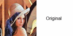
在我们开始图像处理方法之旅之前,我们应该简要了解一位特定模特和她的照片的故事。

对于从事图像处理的人来说,这张照片很熟悉。上图显示了瑞典模特 Lenna Soderberg(née Sjööblom)。它最初于1972年11月刊登在《花花公子》的插页上。
这张照片最早于1973年偶然使用,从那时起,它就成为了图像处理和压缩研究中最重要的照片。
数字世界中的图像表示
我们每天观察的世界是连续的。这就是我们的眼睛感知图像的方式。要在数字媒体上捕捉模拟图像,需要对其进行采样和量化——简而言之,需要对其进行数字化。
采样
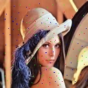
作为连续二维信号(图像)采样的结果,我们得到一个具有定义行数和列数的离散二维信号。位于给定行和列交点的点(元素)称为像素。原始图像的采样是一种有损操作——采样图像的质量取决于设定的采样级别。


图。使用不同采样级别后的结果。
量化
量化是回答我们离散图像中每个像素值是多少的操作。典型的量化级别是 2、64、256、1024、4096、16384。例如,如果我们使用 1024 个量化级别,则意味着每个像素的值是在 0 到 1024 范围内的自然数。


图。使用不同量化级别后的结果。
Color
我们需要添加到数字图像中的最后一个信息是每个像素的颜色。最流行的颜色模型是立方体 RGB 模型。红色、绿色和蓝色是我们能够创建任何其他颜色的颜色。在 RGB 模型中,每个图像像素由三个值描述——每种颜色的饱和度。

另一种常见的颜色模型是 HSV。HSV 模型使用三个分量描述颜色:色相 (hue)、饱和度 (saturation) 和值 (value)。该模型可以被视为一个圆锥体,其底部是调色板。

在印刷过程中,最流行的颜色模型是 CMYK,它代表四种原色:青色 (cyan)、品红色 (magenta)、黄色 (yellow) 和黑色 (key)。在印刷过程中,每种颜色元素组合在一起以产生最终颜色。

直方图
图像直方图是图像中每种颜色或亮度级别出现次数的统计信息。直方图告诉我们很多关于图像的信息——不仅仅是其亮度和对比度。使用直方图,我们可以推断图像细节是否被正确捕获和存储。
分析彩色图像时,我们会为每种颜色 (RGB) 得到直方图。对于灰度图像,可以生成单个直方图。


图。彩色和灰度图像的直方图。
频域中的图像表示 - 图像频谱
离散傅立叶变换
图像应被视为任何其他在离散空间域中传输信息的信号。因此,我们可以将其转换为频域。
离散正向和反向傅立叶变换(正向 DFT、反向 DFT)用公式描述:
从上面我们可以注意到,F(0,0) 指的是静态分量。从这个点开始,表示了更高的频率。我们需要记住,每个复数都可以表示为幅度 (magnitude) 和相位 (phase)。
尽管信息仅由幅度携带,但为了能够计算反变换,我们仍然需要记住相位分量。为了将幅度表示为位图,我们还需要对其值进行归一化。通常我们使用对数尺度进行归一化。


图。图像 DFT 的幅度。
通常假设静态分量显示在图像的中间。因此,我们需要执行频谱移位。
而不是进行移位操作,可以在原始图像上进行。请注意,

图。图像 SDFT 的幅度。我们可以看到幅度在所有频率范围内都达到非零值,尽管静态分量占主导地位。我们还可以注意到,图像中有三个方向(垂直、水平和 45º 斜线)占主导地位。
A. 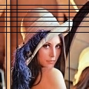

B. 

C. 

D. 

图。图像的变化如何影响其频谱。A. 添加额外的水平线和垂直线增强了频谱中的这些方向。B. 添加低级噪声导致可见频谱的主要方向被抑制。C. 添加高级噪声导致所有频率的幅度值模糊。D. 旋转图像导致频谱中的主要方向旋转。
基本图像转换
颜色模型转换
下方的公式显示了三种最常见颜色模型之间的转换思路。
RGB 转 HSV
辅助变量
最终计算
HSV 转 RGB
辅助变量
最终计算
1. 如果 IH(x,y) 在 0º 和 60º 之间
2. 如果 IH(x,y) 在 60º 和 120º 之间
3. 如果 IH(x,y) 在 120º 和 180º 之间
4. 如果 IH(x,y) 在 180º 和 240º 之间
5. 如果 IH(x,y) 在 240º 和 300º 之间
6. 如果 IH(x,y) 在 300º 和 360º 之间
RGB 转 CMYK
RGB 颜色分量归一化
各个 CMYK 分量的计算


图。青色、品红色、黄色和黑色图层。
CMYK 转 RGB
各个 RGB 分量的计算
彩色图像转灰度
有几种算法可以将彩色图像转换为灰度图像。它们之间的区别在于将三个颜色分量转换为一个亮度值的方法。
平均法
最终结果是每个颜色分量的平均值。
亮度法
最终结果是颜色分量的最大值和最小值的平均值。
亮度感度法
最流行的方法,旨在匹配我们对亮度的感知。这种方法使用颜色分量的加权组合。


图。灰度化操作的结果(从左到右:平均法、亮度法、亮度感度法)。

图。灰度化操作之间的差异。
灰度图像转黑白
将灰度图像转换为黑白图像,就是检查每个像素的亮度值是否低于或高于设定的阈值 T。


图。使用不同阈值转换的图像(从左到右:100、128、156)。
负片
在计算负片图像时,我们计算每个像素的补数。这是一个可逆操作,即双重使用此函数的结果是原始图像。
对于彩色图像,每个颜色分量都应使用上述公式计算。


图。正片和负片图像。
反转
计算反转图像涉及计算每个像素的新值,该值相对于转换点对称。


图。反转的灰度图像(转换点 128)。


图。反转的黑白图像(转换点 128)。
加法
两个图像的相加就像两个数字的相加一样简单。
由于可用的亮度值,需要检查附加条件。

图。图像 A。

图。图像 B。
图。A + B。
减法
减去两个图像时,我们需要注意哪个图像是被减数,哪个是减数。
与图像加法一样,需要检查可用的亮度值条件。

图。图像 A。

图。图像 B。

图。B - A。
水平和垂直翻转
这些操作会创建图像的镜像反射。
Horizontal
其中 W 是图像宽度。


图。水平翻转。
垂直
其中 H 是图像高度。

图。垂直翻转。
对比度拉伸
对比度拉伸是基于直方图的操作之一。当其直方图主要分布在左侧时,我们使用它来增强原始图像。其思想是拉伸(增加)整个可用范围的对比度。
该操作由以下公式描述:
其中 IMIN 和 IMAX 是图像中的最小和最大亮度值,MIN 和 MAX 是输出直方图中最小和最大可用值。


图。原始图像。


图。对比度拉伸(Min = 0, Max = 255)。


图。对比度拉伸(Min = 50, Max = 255)。
直方图平移
直方图平移操作用于增强或减暗。它只是将偏移值添加到每个像素。


图。原始图像。


图。直方图平移图像(偏移量 = 75)。
直方图均衡化
当图像对比度低时,使用直方图均衡化方法。其思想是展开图像直方图以增强对比度并突出图像主体和背景之间的差异。
操作由以下公式描述:
其中 H 是可用的亮度级别(通常是 256),pi 是具有特定亮度值的像素的出现概率。
其中 hist(i) 表示具有 i 级亮度的像素数量(i 是直方图向量的元素),N 表示图像中的总像素数。
此操作经常用于投影仪中,作为提高显示图像质量的方法。


图。原始图像。


图。直方图均衡化图像。
对数缩放
对数缩放操作通过替换为像素值的对数来归一化像素值。结果是较低的值得到增强,整个直方图被拉伸。
通常我们使用 10 为底或自然对数。该操作由以下公式描述:


图。原始图像。


图。对数缩放图像。
工作区更改
工作区更改操作(有时称为画布更改)包括更改(减小或扩展)图像大小而不更改原始图像像素值。
我们需要定义的第一个是感兴趣区域的锚点位置。在图像裁剪操作中,锚点位置定义了新的裁剪位置;在图像补操作中,锚点位置定义了新尺寸中原始图像的位置。

图。锚点位置。
裁剪
在图像裁剪操作中,新的感兴趣区域的起始点 (x1; y1) 需要根据假定的锚点位置来计算。
设 W 和 H 为原始图像的尺寸(宽度和高度),设 w 和 h 为裁剪图像的尺寸。那么:
中心
西
东
北
南
西北
东北
西南
东南
最后,对于新图像的每个像素,我们取原始图像的相应像素。

图。原始图像(225 x 225 像素)。


图。裁剪的图像 50 x 50 像素(从左锚点位置:西、中、北、西北、东北、南、西南、东南、东)。
补集
在图像补操作中,新的感兴趣区域的起始点 (x1; y1) 和结束点 (x2; y2) 需要根据假定的锚点位置来计算。
设 W 和 H 为补图像的尺寸(宽度和高度),设 w 和 h 为原始图像的尺寸。那么:
中心
西
东
北
南
西北
东北
西南
东南
最后


图。原始图像(125 x 125 像素)和补图像(150 x 150 像素)以及中心锚点位置。
重采样
重采样操作包括更改处理后的图像中的像素数量,以调整其大小、更改比例或旋转。
调整大小
在调整大小时,我们希望更改图像的宽度和高度,无论是否保持其比例。我们将原始图像的宽度和高度表示为W、H,将期望的宽度和高度表示为WO 和 HO。
因此,变换比例为:
最近邻
这是最简单的图像缩放方法。
对于每个像素,我们需要计算其在原始图像中的对应像素。


图。使用最近邻方法调整图像大小(从左到右:原始 128x128,缩放到 256x256 和 50x50)。
双线性插值
最近邻方法的缺点是在图像中留下锯齿状边缘。这个问题可以通过涉及周围像素插值的方法来解决。
对于每个像素,我们需要计算原始图像中感兴趣区域的中心。


图。使用双线性插值法调整图像大小(从左到右:原始 128x128,缩放到 256x256 和 50x50)。

图。两种方法的比较。
旋转
要旋转图像,我们需要选择旋转中心 (xc, yc)——我们将在其周围转换图像的点。这通常是原始图像的中心,但此处演示的变换允许选择任意点。
输出图像的像素(x, y) 是原始图像的像素 (xA, yA),计算如下:


图。图像旋转(从左到右 30º、45º、60º),图像中心是旋转中心。

图。图像旋转 30º,旋转中心位于点 x=25, y=25。
线性滤波
线性滤波不过是频率滤波,其中某些频率保持不变,而其他频率被抑制。滤波操作可以在频域和空域中进行。
在计算复杂度方面,在空域进行滤波要容易得多(无需计算正向和反向傅立叶变换),但必须记住,频率滤波器是在频域中描述的,并且在空域中找到这种滤波器的核并不总是容易的方法。
空域卷积
在空域中,频率滤波器由实值矩阵表示。要获得输出图像,我们需要计算原始图像与滤波器掩码的二维卷积。
3x3 维度的滤波器可以表示为矩阵:
其中中心元素x5 对应于输出像素的计算位置。滤波器掩码通过以下操作在原始图像的所有行和列中“移动”:
对于彩色图像,我们需要为每个图层执行上述操作。
低通滤波器
低通滤波器(有时称为平均滤波器)抑制高频并保留低频。它通过组合两个一维滤波器来构建。


图。一维和二维低通滤波器。蓝色表示通带。
实际上,低通滤波是计算每个输出滤波器的平均值。不期望的效果是图像模糊。低通滤波器掩码的例子是:


图。低通滤波(从左到右:原始、LPF1、LPF2、LPF3、LPF4)。
高通滤波器
高通滤波器(有时称为锐化滤波器)抑制低频并保留高频。它通过组合两个一维滤波器来构建。


图。一维和二维高通滤波器。蓝色表示通带。
这些滤波器的目的是使边缘和小的细节更清晰(在空域中对应高频)。除了期望的效果外,高通滤波器还会加强噪声。高通滤波器掩码的例子是:


图。高通滤波(从左到右:原始、HPF1、HPF2、HPF3、HPF4)。
高斯滤波器
与低通滤波器类似,高斯滤波器可以平滑图像,去除噪声、小的细节并模糊边缘。不同之处在于滤波器掩码的核,在这种情况下,它采用高斯函数的二维图的形式。

图。二维高斯函数。


图。高斯滤波器(从左到右:原始、GF1、GF2、GF3)。
非线性滤波
非线性滤波器是另一类滤波。与线性滤波器不同,我们不能使用卷积来计算输出图像(因此不能在频域中处理图像)。因此,非线性滤波算法比线性算法慢。然而,使用非线性滤波器在初始图像处理中可以取得良好的效果。
中值滤波器
中值滤波器是最流行的非线性滤波器。在该操作中,为了计算每个像素的新值,我们取最近邻域像素的中值。最近邻域的范围由滤波器掩码大小定义。使用较大尺寸的掩码会导致输出图像的模糊度更大。
使用 3x3 掩码进行中值滤波的步骤如下:
1. 获取最近邻域像素值。
2. 将这些值从最小值到最大值排序。
3. 计算新像素值作为上述列表的中值,即s5 元素。


图。彩色图像的中值滤波(从左到右:原始图像、3x3 掩码、5x5 掩码)。
中值滤波用于脉冲(椒盐)噪声抑制。与低通滤波器不同,中值滤波器在平滑亮度值变化时造成的损害较小。


图。使用 3x3 中值滤波器进行脉冲噪声抑制。
信号相关排序均值滤波器 (SD ROM)
中值滤波器的缺点是即使像素未损坏也会改变其值。结果是我们的图像会变模糊,而不考虑它是否受到噪声干扰。SD ROM 滤波器的思想是检查像素是否损坏,仅在此情况下计算其新值。
使用 3x3 掩码进行 SD ROM 滤波的步骤如下:
1. 获取最近邻域像素值。
2. 将这些值从最小值到最大值排序。
3. 计算排序均值。
4. 计算排序差值向量。
其中对于声明的掩码尺寸 3x3,i = 1, 2, 3, 4。
5. 对于 ROD 向量中的每个元素,检查条件:
其中
并且 T 是一个给定的阈值向量,其中:
如果第 5 点中的任何一个条件为真,我们可以假定像素 (x, y) 已损坏,并将其值更改为 ROM(x,y)。否则,我们将其值保留为原始图像中的值。
对于 N x N 掩码的一般情况,我们的
1A. 最近邻像素值矩阵将是 N x N。
2A. R 向量将有 N2 - 1 个元素。
3A. 排序均值计算将是:
4A. 排序差值向量计算将是:
其中 i = 1, 2, 3, 4, ..., (N2 - 1) / 2。
5A. 我们需要声明 N2 - 1 个阈值向量元素。


图。彩色图像的 SD ROM 滤波(从左到右:原始图像、3x3 掩码、5x5 掩码)。


图。使用 3x3 SD ROM 滤波器进行脉冲噪声抑制。
图。比较使用中值和 SD ROM 滤波器进行噪声抑制。
川岛滤波器
川岛滤波器是另一种平滑算子,它不像中值滤波器那样模糊图像边缘,但与 SD ROM 滤波器相反,它会改变每个计算像素的值。
为了计算像素p(x,y) 的值,我们的感兴趣区域是尺寸为 (2N-1) x (2N-1) 的最近邻域,其中N 表示川岛滤波器的尺寸。对于N = 3,我们得到感兴趣区域:
下一步,我们将上述掩码分成四个更小的、尺寸为N x N 的子掩码。
对于每个掩码,我们计算均值和方差。
p(x,y) 的新值是方差最小的掩码的均值。


图。使用尺寸为 3 的川岛滤波器进行脉冲噪声抑制。
形态滤波
形态滤波应被视为图像处理的一个完全独立的分支。它主要用作预处理,为进一步操作准备图像。通常,形态学方法用于二值图像的处理,但也可以成功用于灰度图像的处理。
然而,使用形态滤波器处理彩色图像并非易事,因为像素各个颜色分量之间存在很强的相关性——单独过滤每个颜色层然后连接起来并不能给我们带来满意的结果。
本文将重点介绍形态学操作在二值图像处理中的最常见用法。
腐蚀
此滤波器的目的是侵蚀图像中的紧凑对象,以消除与相邻对象的意外连接或对象的锯齿状边缘。
在该操作中,为了计算每个像素的新值,我们取最近邻域像素的最小值。最近邻域的范围由滤波器掩码大小定义。
使用 3x3 掩码进行腐蚀滤波的步骤如下:
1. 获取最近邻域像素值。
2. 计算新像素值,即上述矩阵的最小值。


图。图像腐蚀(从左到右:原始图像、3x3 掩码腐蚀、5x5 掩码腐蚀)。
膨胀
此滤波器的目的是使对象表面变粗,以消除凹陷。
在该操作中,为了计算每个像素的新值,我们取最近邻域像素的最大值。最近邻域的范围由滤波器掩码大小定义。
使用 3x3 掩码进行腐蚀滤波的步骤如下:
1. 获取最近邻域像素值。
2. 计算新像素值,即上述矩阵的最大值。


图。图像膨胀(从左到右:原始图像、3x3 掩码膨胀、5x5 掩码膨胀)。
开运算
正如腐蚀滤波效果图所示,使用适当的掩码尺寸可以分离四个对象。然而,不期望的效果是每个对象的面积减小。
为了避免这种情况,通常不使用腐蚀滤波,而是使用开运算,即用腐蚀掩码过滤后的图像进行膨胀。


图。图像开运算(腐蚀和膨胀均使用 5x5 掩码)。
闭运算
与腐蚀中观察到的效果相反,图像膨胀的结果可以看到。凹陷消失了,但对象填充区域增大了。
为了避免这种情况,我们可以使用闭运算,即用膨胀掩码过滤后的图像进行腐蚀。


图。图像闭运算(膨胀和腐蚀均使用 5x5 掩码)。
骨架化
最常见的定义,或者说骨架化的目的,是提取基于区域的形状特征,代表图像对象的通用形式。结果是我们接收给定对象的中心轴。
对象的骨架并不唯一——两个不同的形状可以具有相同的骨架。

图。二值图像及其骨架。
骨架化算法可以分为三个步骤:
步骤 1. 图像准备。
如果我们假设二值图像的像素值为 0(黑色)和 1(白色),则此步骤可以省略。否则,在此步骤中所要做的就是将像素值归一化为 0 和 1。
步骤 2. 递归计算中心轴方向。
为了计算下一个值,我们遵循以下公式:
应重复计算,直到表中不再发生变化。
步骤 3. 骨架线隔离。
骨架线可以用以下公式计算:
边缘检测滤波
图像处理中的典型案例是边缘检测——在医学图像处理中非常常用。空间域的边缘检测可以分为使用定向或非定向滤波器进行的操作。
定向滤波需要双倍的数学运算并进一步组合结果。非定向滤波器则不需要。
边缘检测滤波也称为导数滤波或梯度滤波,因为它基于确定原始图像的导数。通常,边缘的出现是像素亮度级别的突然变化,这在第一(或后续)导数的值上得到强烈反映。
Sobel 滤波器
Sobel 滤波器,或 Sobel 算子,是定向滤波器的示例。
它使用掩码检测水平边缘:
以及使用以下掩码检测垂直边缘:
最后,我们组合结果:
这可以近似为:


图。使用 Sobel 滤波器对彩色图像进行边缘检测。

图。使用 Sobel 滤波器对灰度图像进行边缘检测。


图。使用 Sobel 滤波器对非自然黑白图像进行边缘检测。
Prewitt 滤波器
Prewitt 滤波器,或 Prewitt 算子,是定向滤波器的示例。
水平掩码:
垂直掩码:


图。使用 Prewitt 滤波器对彩色图像进行边缘检测。


图。使用 Prewitt 滤波器对灰度图像进行边缘检测。


图。使用 Prewitt 滤波器对非自然黑白图像进行边缘检测。
拉普拉斯滤波器
使用拉普拉斯掩码的滤波是计算二阶导数。这些是非定向滤波器的例子。拉普拉斯掩码的例子如下所示:


图。使用拉普拉斯滤波器对彩色图像进行边缘检测。


图。使用拉普拉斯滤波器对灰度图像进行边缘检测。


图。使用拉普拉斯滤波器对非自然黑白图像进行边缘检测。
艺术滤镜和处理
彩色滤波
这是一个非常简单的算法,可以替代相机镜头上使用的物理滤镜。
自然光(由对应不同颜色的不同波长组成)穿过彩色滤镜时会丢失(抑制)选定的波长。结果是只有选定的颜色(波长)才能到达图像传感器。
例如,当使用品红色滤镜时,品红色由红色和蓝色组成,只有红色和蓝色分量会通过——绿色将被阻挡。


图。彩色滤波(从左上角开始的滤镜颜色:青色、品红色、黄色、青品红、品红黄、黄青)。
伽马校正
伽马校正用于减小或增大对比度。
对于灰度图像,它由以下公式给出:
其中 INOR 表示归一化到 0-1 范围的图像值。
对于彩色图像,上述操作应为每个颜色分量重复执行。


图。伽马校正(从左到右:0.25、0.5、0.75、1.5、2)。
棕褐色
棕褐色调是传统摄影处理中使用的一种技术。这项技术被用于延长照片印刷品的寿命。结果是图像呈现棕褐色。
要通过数字图像处理获得相同的效果,需要执行两个操作:首先,我们将彩色图像转换为灰度,然后我们使用以下公式更改每个像素的 RGB 值:


图。不同级别的棕褐色图像(从左到右:10、20、30、40、80)。
色彩强调
这种艺术技术基于强调(保留)图像中选定的颜色,而将所有其他颜色转换为灰度。
为此,我们将使用 HSV 颜色模型而不是 RGB 模型。这要容易得多,因为在 HSV 模型中我们可以只关注一个颜色参数——色相。当然,色相值可能不同,因此我们应该假定一个可接受的变化范围。
让我们表示我们想要强调的颜色的色相值h,以及可接受的范围r。我们可以计算值:
这些值可以具有以下关系:
1.
在这种情况下,如果此外还满足:
2.
在这种情况下,如果此外还满足:


图。色彩强调示例。
图层
图层是图像处理中非常常见的操作。结果是我们得到一个结合了两个输入(背景和图层)的图像。
为了计算输出像素,我们使用一种称为 Alpha 混合的技术,该技术由以下公式给出:
最后,我们计算(x, y) 像素的新 alpha 因子。


图。添加图层示例。
移轴
移轴技术在传统摄影中很受欢迎,通过使用具有光学轴移可能性的特殊镜头,我们可以改变图像透视。最终我们得到一个看起来像模型的图像。
在数字图像处理中,我们可以在没有专业摄影设备的情况下获得相同的结果。
移轴图像分为三个部分:其中两个是模糊的,中间部分保持与原始图像一样清晰。比例可以变化,在我们使用的例子中,我们采用“一半一半”的技术,其中顶部模糊部分是原始图像的一半,底部模糊部分是左半部分的一半。

图。移轴图像结构。
为了模糊图像,我们将使用一维高斯滤波器。模糊可以水平或垂直进行。高斯函数如下所示:
其中
L - 是靠近锐化部分的模糊定义的函数值(例如,在 0.05 - 0.15 的范围内)。
S - 是靠近模糊部分的模糊定义的函数值(例如,在 5 - 7 的范围内)。
n - 是计算像素与锐化部分之间的距离。
N0.5 - 是较大模糊区域的高度(在垂直模糊中)。
对于每个需要模糊的像素,我们执行计算(垂直模糊):
为了使上述公式可计算,我们需要将低值的高斯滤波器(例如,低于 0.005 的值)视为可忽略。


图。移轴效果。
图像模糊
图像模糊操作与移轴滤波非常相似。我们可以使用相同的高斯函数作为模糊算子。区别在于输出图像结构,我们在此定义一个锐环的中心及其半径。此环外面的所有像素都应被模糊。

图。模糊图像结构。
计算特定像素与环中心之间的距离的公式如下:
如果r > R,我们使用高斯滤波器。

图。模糊图像(中心位于点 250x180,半径 80)。
模糊背景
当将图像(旋转或不旋转)放置在由同一图像但模糊的版本创建的背景上时,可以获得有趣的效果。以下操作是:
1. 使用高斯滤波器模糊图像(此步骤可以重复两次或三次)- 此模糊图像将是我们的背景。
2. 补全图像(原始图像)并添加白色边框。
3. 补全 2 的结果,添加透明背景(以去除“狗耳朵”)。
4. 旋转 3 的结果(如果我们不想旋转前景,可以跳过步骤 3 和 4)。
5. 将前景图像作为图层添加到背景中。


图。模糊背景效果。
宝丽来相框效果
宝丽来相框效果类似于模糊背景合成。通过省略背景创建并增大底部边框宽度,我们可以获得它。
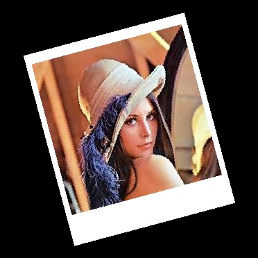
图。宝丽来相框效果。
铅笔素描
铅笔素描效果可以通过组合两个操作获得:边缘检测和黑白反转(根据定义的强度)。
我们还可以使用 SD-ROM 算法来处理较小的伪影而不模糊边缘。


图。铅笔素描效果(拉普拉斯边缘检测,80 以上的黑白反转,SD-ROM)。
炭笔素描
炭笔效果的获得方式与铅笔素描类似。此外,我们可以在开始和结束时平滑图像(中值或高斯滤波器)。而不是使用黑白方法,我们可以使用图像反转算子。


图。炭笔效果(Sobel 边缘检测,80 值反转,5 尺寸的中值平滑)。
油画
为了获得油画效果,我们需要减少像素强度的可用级别。通常,每个像素由 256 个强度级别描述——对于油画滤波,我们将减少它们十倍以上。
为了对像素进行分类,我们需要考虑其在定义的半径(油画滤波器大小)r 的最近邻域中的强度。此外,我们用L 表示定义的可用强度级别。
我们表示强度级别出现次数的向量:I - 分类强度的直方图,R, G, B - 分类强度下的红色、绿色和蓝色值。
对于定义为r 的邻域中的每个像素,我们计算分类强度:
并递增向量:
之后,我们确定直方图I 的最大值及其最大值的索引k。
最后,我们计算新的红色、绿色和蓝色值,如下:


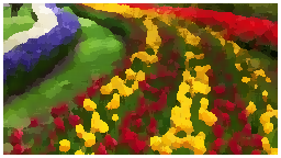
图。油画效果(半径为 7 的滤波器,15 级颜色强度)。
卡通效果
如果我们在此基础上结合油画滤波结果和反向边缘检测滤波,我们可以获得同样有趣的效果——图像看起来像漫画书。


图。卡通效果(油画滤波器半径为 7,10 级颜色强度,反转阈值 40,Sobel 算子)。
使用代码
本文介绍的所有图像处理算法都已在随附的源代码中实现。要开始使用 FIP 库,只需声明其命名空间。
using FIP;
创建新对象
FIP.FIP fip = new FIP.FIP(); // many "fip's" in one line...
并开始您的数字图像处理之旅……
调用库方法
直方图
获取直方图表
Bitmap img = new Bitmap("781213/lena.jpg");

int[] greyscaleHistogram = fip.Histogram(img); // Greyscale histogram
int[,] rgbHistogram = fip.RGBHistogram(img); // RGB histogram
离散傅立叶变换
正向傅立叶变换
Bitmap img = new Bitmap("781213/lena.jpg");

Complex[,] spectrum = fip.DFT(img); // Basic forward Fourier Transform

Complex[,] spectrumShifted = fip.SDFT(img); // Forward Fourier Transform with shift operation
获取幅度和相位
Double[,] magnitude = fip.Magnitude(spectrum);

Double[,] phase = fip.Phase(spectrum);
反向傅立叶变换
Bitmap inv = fip.iDFT(spectrum); // To Bitmap

Double[,] invTab = fip.iDFT2(spectrum); // To table
如果应用了移位操作
Bitmap inv = fip.iSDFT(spectrum); // To Bitmap

Double[,] invTab = fip.iSDFT2(spectrum); // To table
颜色模型转换
Bitmap img = new Bitmap("781213/lena.jpg");

Color pixel = img.GetPixel(1, 1); // Get single pixel

Double[] hsv = fip.rgb2hsv(pixel); // Single pixel convertion from RGB to HSV
Color pixel2 = fip.hsv2rgb(hsv); // Single pixel convertion from HSV to RGB

Double[] cmyk = fip.rgb2cmyk(pixel); // Single pixel convertion from RGB to CMYK
Color pixel3 = fip.cmyk2rgb(cmyk); // Single pixel convertion from CMYK to RGB

Bitmap[] CMYKLayers = fip.CMYKLayers(img); // Get CMYK Layers form ARGB image

Bitmap[] RGBLayers = fip.RGBLayers(img); // Get RGB Layers as bitmaps
int[,,] RGBLayers2 = fip.RGBMatrix(img); // Get RGB Layers as tables

int[,] RLayer = fip.RMatrix(img); // Get red color layer
int[,] GLayer = fip.GMatrix(img); // Get green color layer
int[,] BLayer = fip.BMatrix(img); // Get blue color layer
转换为灰度
Bitmap img = new Bitmap("781213/lena.jpg");

Color pixel = img.GetPixel(1, 1); // Get single pixel

Color pixelGS = fip.color2greyscale(pixel); // Single pixel convertion using luminance method

Bitmap average = fip.ToGreyscaleAVG(img); // Average method of greyscaling
Bitmap lightness = fip.ToGreyscaleLightness(img); // Lightness method of greyscaling
Bitmap luminance = fip.ToGreyscale(img); // Luminance method of greyscaling
转换为黑白
Bitmap img = new Bitmap("781213/lena.jpg");

Bitmap bw = fip.ToBlackwhite(img, 128); // Convert to black and white with threshold on 128
Bitmap bwinv = fip.ToBlackwhiteInverse(img, 80); // Convert to black and white with threshold on 80 and invert over this point
负片
Bitmap img = new Bitmap("781213/lena.jpg");

Bitmap negative = fip.NegativeImageColor(img); // Color image negative
Bitmap negativeGS = fip.NegativeImageGS(img); // Converts to greyscale and negative transform
反转
Bitmap img = new Bitmap("781213/lena.jpg");

Bitmap inverse = fip.InverseImage(img, 190); // Inverse image on point 190
图像加法和减法
Bitmap a = new Bitmap("a.jpg");
Bitmap b = new Bitmap("b.jpg");

Bitmap c = fip.AddImages(a, b); // Add two images
Bitmap d = fip.SubtractImages(a, b); // subtract two images a - b
水平和垂直翻转
Bitmap img = new Bitmap("781213/lena.jpg");

Bitmap mirrorvertical = fip.FlipVertical(img);
Bitmap mirrorhorizontal = fip.FlipHorizontal(img);
对比度拉伸
Bitmap img = new Bitmap("781213/lena.jpg");

Bitmap contraststretching = fip.ContrastStretching(img); // Contrast stretching in whole range
Bitmap contraststretching2 = fip.ContrastStretching(img, 50, 255); // Contrast stretching in range 50 - 255
直方图平移
Bitmap img = new Bitmap("781213/lena.jpg");

Bitmap histshift = fip.HistogramShift(img, 50); // Histogram shift with threshold of 50
直方图均衡化
Bitmap img = new Bitmap("781213/lena.jpg");

Bitmap histeq = fip.HistoramEqualization(img);
对数缩放
Bitmap img = new Bitmap("781213/lena.jpg");

Bitmap logscale = fip.LogaritmicScaling(img); // Logarithmic scaling with 10-base logarithm
裁剪图像
Bitmap img = new Bitmap("781213/lena_cut.jpg");
Bitmap cut = fip.ImageCut(img, 50, 50, FIP.FIP.Anchor.Middle);
补集图像
Bitmap img = new Bitmap("781213/lena_complement.jpg");
Bitmap complement = fip.ImageComplement(img, 150, 150, Color.FromArgb(255, 0, 0, 0), FIP.FIP.Anchor.Middle);
图像调整大小
Bitmap img = new Bitmap("781213/lena.jpg");

Bitmap img2 = fip.Resize(img, 50, 50); // Image resize with nearest neighbourhood method
Bitmap img3 = fip.Resize2(img, 50, 50); // Image resize with bilinear interpolation method
图像旋转
Bitmap img = new Bitmap("781213/lena.jpg");

Bitmap rotate = fip.Rotate(img, 30); // Image rotation over 30 degrees
线性滤波器示例
低通滤波器
        /// <summary>
        /// Low pass filter
        /// </summary>
        /// <returns>Low pass filter</returns>
        public Double[,] LPF1()
        {
            return new Double[3, 3] { { 0.1111, 0.1111, 0.1111 }, { 0.1111, 0.1111, 0.1111 }, { 0.1111, 0.1111, 0.1111 }, };
        }

        /// <summary>
        /// Low pass filter
        /// </summary>
        /// <returns>Low pass filter</returns>
        public Double[,] LPF2()
        {
            return new Double[3, 3] { { 0.1, 0.1, 0.1 }, { 0.1, 0.2, 0.1 }, { 0.1, 0.1, 0.1 }, };
        }

        /// <summary>
        /// Low pass filter
        /// </summary>
        /// <returns>Low pass filter</returns>
        public Double[,] LPF3()
        {
            return new Double[3, 3] { { 0.0625, 0.125, 0.0625 }, { 0.125, 0.25, 0.125 }, { 0.0625, 0.125, 0.0625 }, };
        }

        /// <summary>
        /// Low pass filter
        /// </summary>
        /// <returns>Low pass filter</returns>
        public Double[,] LPF4()
        {
            return new Double[5, 5] {
            { 0.00366, 0.01465, 0.02564, 0.01465, 0.00366 },
            { 0.01465, 0.05861, 0.09524, 0.05861, 0.01465 },
            { 0.02564, 0.09524, 0.15018, 0.09524, 0.02564 },
            { 0.01465, 0.05861, 0.09524, 0.05861, 0.01465 },
            { 0.00366, 0.01465, 0.02564, 0.01465, 0.00366 }
            };
        }
高通滤波器
        /// <summary>
        /// High pass filter
        /// </summary>
        /// <returns>High pass filter</returns>
        public int[,] HPF1()
        {
            return new int[3, 3] { { -1, -1, -1 }, { -1, 9, -1 }, { -1, -1, -1 }, };
        }

        /// <summary>
        /// High pass filter
        /// </summary>
        /// <returns>High pass filter</returns>
        public int[,] HPF2()
        {
            return new int[3, 3] { { 0, -1, 0 }, { -1, 5, -1 }, { 0, -1, 0 }, };
        }

        /// <summary>
        /// High pass filter
        /// </summary>
        /// <returns>High pass filter</returns>
        public int[,] HPF3()
        {
            return new int[3, 3] { { 1, -2, 1 }, { -2, 5, -2 }, { 1, -2, 1 }, };
        }

        /// <summary>
        /// High pass filter
        /// </summary>
        /// <returns>High pass filter</returns>
        public int[,] HPF4()
        {
            return new int[5, 5] {
            { -1, -1, -1, -1, -1 },
            { -1, -1, -1, -1, -1 },
            { -1, -1, 25, -1, -1 },
            { -1, -1, -1, -1, -1 },
            { -1, -1, -1, -1, -1 }
            };
        }
高斯滤波器
        /// <summary>
        /// Gausian filter
        /// </summary>
        /// <returns>Gausian filter</returns>
        public Double[,] GF1()
        {
            return new Double[3, 3] { { 0.0625, 0.125, 0.0625 }, { 0.125, 0.25, 0.125 }, { 0.0625, 0.125, 0.0625 }, };
        }

        /// <summary>
        /// Gausian filter
        /// </summary>
        /// <returns>Gausian filter</returns>
        public Double[,] GF2()
        {
            return new Double[5, 5] {
            { 0.0192, 0.0192, 0.0385, 0.0192, 0.01921 },
            { 0.0192, 0.0385, 0.0769, 0.0385, 0.0192 },
            { 0.0385, 0.0769, 0.1538, 0.0769, 0.0385 },
            { 0.0192, 0.0385, 0.0769, 0.0385, 0.0192 },
            { 0.0192, 0.0192, 0.0385, 0.0192, 0.0192 }
            };
        }

        /// <summary>
        /// Gausian filter
        /// </summary>
        /// <returns>Gausian filter</returns>
        public Double[,] GF3()
        {
            return new Double[7, 7] {
            { 0.00714, 0.00714, 0.01429, 0.01429, 0.01429, 0.00714, 0.00714 },
            { 0.00714, 0.01429, 0.01429, 0.02857, 0.01429, 0.01429, 0.00714 },
            { 0.01429, 0.01429, 0.02857, 0.05714, 0.02857, 0.01429, 0.01429 },
            { 0.01429, 0.02857, 0.05714, 0.11429, 0.05714, 0.02857, 0.01429 },
            { 0.01429, 0.01429, 0.02857, 0.05714, 0.02857, 0.01429, 0.01429 },
            { 0.00714, 0.01429, 0.01429, 0.02857, 0.01429, 0.01429, 0.00714 },
            { 0.00714, 0.00714, 0.01429, 0.01429, 0.01429, 0.00714, 0.00714 }
            };
        }
拉普拉斯滤波器
        /// <summary>
        /// Laplace filter
        /// </summary>
        /// <returns>Laplace filter</returns>
        public int[,] LaplaceF1()
        {
            return new int[3, 3] { { -1, -1, -1 }, { -1, 8, -1 }, { -1, -1, -1 }, };
        }

        /// <summary>
        /// Laplace filter
        /// </summary>
        /// <returns>Laplace filter</returns>
        public int[,] LaplaceF2()
        {
            return new int[3, 3] { { 0, -1, 0 }, { -1, 4, -1 }, { 0, -1, 0 }, };
        }

        /// <summary>
        /// Laplace filter
        /// </summary>
        /// <returns>Laplace filter</returns>
        public int[,] LaplaceF3()
        {
            return new int[3, 3] { { 1, -2, 1 }, { -2, 4, -2 }, { 1, -2, 1 }, };
        }

        /// <summary>
        /// Laplace filter
        /// </summary>
        /// <returns>Laplace filter</returns>
        public int[,] LaplaceF4()
        {
            return new int[5, 5] {
            { -1, -1, -1, -1, -1 },
            { -1, -1, -1, -1, -1 },
            { -1, -1, 24, -1, -1 },
            { -1, -1, -1, -1, -1 },
            { -1, -1, -1, -1, -1 }
            };
        }
线性滤波
Bitmap img = new Bitmap("781213/lena.jpg");

Bitmap fitered = fip.ImageFilterColor(img, fip.LaplaceF1()); // Image filtration with Laplace filter no 1
Bitmap fiteredGS = fip.ImageFilterGS(img, fip.LaplaceF1()); // Image filtration (with greyscaling operation) with Laplace filter no 1
中值滤波器
Bitmap img = new Bitmap("781213/lena.jpg");

Bitmap median = fip.ImageMedianFilterColor(img, 5); // Median filtration with mask size 5;
Bitmap medianGS = fip.ImageMedianFilterGS(img, 5); // Median filtration with greyscaling and filter mask size 5
SD-ROM 滤波器
Bitmap img = new Bitmap("781213/lena.jpg");

Bitmap sdrom = fip.ImageSDROMFilterColor(img); // SD ROM filtration with parameters described in article
Bitmap sdrom2 = fip.ImageSDROMFilterColor(img, 3, new int[4] { 30, 40, 50, 60 }); // SD ROM filtration with given parameters

Bitmap sdromGS = fip.ImageSDROMFilterGS(img); // SD ROM filtration with parameters described in article additionally greyscaling operation

Bitmap sdrom2GS = fip.ImageSDROMFilterGS(img, 3, new int[4] { 30, 40, 50, 60 }); // SD ROM filtration with given parameters additionally greyscaling operation
川岛滤波器
Bitmap img = new Bitmap("781213/lena.jpg");

Bitmap kuwahara = fip.ImageKuwaharaFilterColor(img, 3); // Kuwahara filtartion with mask size 3
腐蚀
Bitmap img = new Bitmap("781213/lena.jpg");

Bitmap erosion = fip.ImageErosionFilterGS(img, 3); // Greyscaling and erosion with mask size 3
膨胀
Bitmap img = new Bitmap("781213/lena.jpg");

Bitmap dilatation = fip.ImageDilatationFilterGS(img, 3); // Greyscaling and dilatation with mask size 3
开运算
Bitmap img = new Bitmap("781213/lena.jpg");

Bitmap open = fip.ImageOpenGS(img, 3); // Opeing with masks size 3
闭运算
Bitmap img = new Bitmap("781213/lena.jpg");

Bitmap close = fip.ImageCloseGS(img, 3); // Closing with masks size 3
骨架化
Bitmap img = new Bitmap("skeletonsource.jpg");

Bitmap skeleton = fip.Skeletonization(img);
Sobel 边缘检测
Bitmap img = new Bitmap("781213/lena.jpg");

Bitmap sobel1 = fip.ImageSobelFilterColor(img); // Sobel edge detecting on color image
Bitmap sobel2 = fip.ImageSobelFilterGS(img); // Sobel edge detecting on greyscale image
Prewitt 边缘检测
Bitmap img = new Bitmap("781213/lena.jpg");

Bitmap prewitt1 = fip.ImagePrewittFilterColor(img); // Prewitt edge detecting on color image
Bitmap prewitt2 = fip.ImagePrewittFilterGS(img); // Prewitt edge detecting on greyscale image
Laplace 边缘检测
Bitmap img = new Bitmap("781213/lena.jpg");

Bitmap laplace1 = fip.ImageFilterColor(img, fip.LaplaceF1()); // Laplace filter no 1 edge detecting on color image
Bitmap laplace2 = fip.ImageFilterGS(img, fip.LaplaceF1()); // Laplace filter no 1 edge detecting on greyscale image
彩色滤波
Bitmap img = new Bitmap("781213/lena.jpg");

Bitmap filteredColor = fip.ColorFiltration(img, "Magenta"); // Color filtration with Magenta filter
可用的彩色滤镜有:品红、黄、青、品红-黄、青-品红、黄-青。
伽马校正
Bitmap img = new Bitmap("781213/lena.jpg");

Bitmap gamma = fip.GammaCorrection(img, 2); // Gamma correction with coefficient 2
棕褐色
Bitmap img = new Bitmap("781213/lena.jpg");

Bitmap sepia = fip.Sepia(img, 30); // Sepia with threshold 30
色彩强调
Bitmap img = new Bitmap("781213/lena.jpg");

Bitmap coloraccent = fip.ColorAccent(img, 140, 50); // Color accent on hue 140 with range 50
图层
Bitmap bg = new Bitmap("781213/lay_lena.jpg");
Bitmap lay = new Bitmap("781213/lay.png");

Bitmap output = fip.AddLayer(bg, lay);
移轴
Bitmap img = new Bitmap("781213/lena.jpg");

Bitmap tiltshift = fip.TiltShift(img); // Tilt shift effect
图像模糊
Bitmap img = new Bitmap("781213/lena.jpg");

Bitmap blur = fip.Blurring(img, 50, 50, 25); // Image bluring out of range 25px from point 50 x 50
模糊背景
Bitmap img = new Bitmap("781213/lena.jpg");

Bitmap lena_bb_0 = fip.BlurredBackground(img, 3, 0.75, 0);
Bitmap lena_bb_30 = fip.BlurredBackground(img, 3, 0.75, 30);
宝丽来相框效果
Bitmap img = new Bitmap("781213/lena.jpg");
Bitmap polaroid = fip.PolaroidFrame(img, 15, 45, 15);
铅笔素描
Bitmap img = new Bitmap("781213/lena.jpg");

Bitmap sketch = fip.Sketch(img); // Pen sketch effect with paramaters from article
炭笔素描
Bitmap img = new Bitmap("781213/lena.jpg");

Bitmap sketch = fip.SketchCharcoal(img); // Charcoal sketch effect with paramaters from article
油画
Bitmap img = new Bitmap("781213/lena.jpg");

Bitmap oilpaint = fip.OilPaint(img, 7, 20); // Oil paint effect, radius 7, 20 levels of intensities
卡通效果
Bitmap img = new Bitmap("781213/lena.jpg");

Bitmap cartoon = fip.Cartoon(img, 7, 10, 40); // Cartoon effect with radius 7, 20 levels of intensities, Sobel edge detecting, inverse on point 40

Bitmap cartoon2 = fip.Cartoon(img, 7, 10, 40, fip.LaplaceF1()); // Cartoon effect with radius 7, 20 levels of intensities, given mask of edge detecting (Laplace), inverse on point 40