Python 傅里叶变换辅助库

• 下载库源码和示例集 - 12.7 KB

引言

Python 3中确实需要一个即插即用的傅里叶变换库，用户可以直接使用并进行傅里叶变换（FT），得到一个经典的、正确缩放的频谱与频率图。

您会发现，商业软件包、开源库、教科书和网络上绝大多数代码都根本不适合这项任务，需要花费数小时的进一步调整才能获得经典的、正确缩放的频谱图。您知道：正确的“幅度”以及不再有“负频率”等。

“傅里叶变换助手库”的作用

FourierTransformHelperLib.py (FTHL) 包含几个主要部分，但其基本目标是允许对实数或复数时间序列输入数组执行真实的傅里叶变换，从而生成一个可用的经典频谱输出，而无需用户进行任何进一步的调整[1]。

提供了许多用例的逐步示例，展示了如何

1. 生成测试信号（稍后可替换为您的真实信号）。
2. 正确应用窗口到输入数据，使用32种包含的窗口中的任何一种。
3. 执行傅里叶变换。
4. 正确缩放傅里叶变换以校正步骤2中应用的窗口。
5. 将傅里叶变换转换为幅度或dBV格式。
6. 绘制漂亮的实数频率幅度显示（即经典的频谱图）

“傅里叶变换助手库”不做什么

在所有这些窗口化、缩放和切片原始傅里叶变换数据以生成可用的仅正频率显示之后，就不可能向后进行正确的傅里叶逆变换了。这是因为傅里叶变换的工作方式。变换的基本数学要求在前向和逆向变换中保持总能量[2]。在所有窗口化、缩放等之后，这必须以某种方式进行回溯才能恢复到原始信号，而这根本不是本库的目的。如上所示，本库的目的是以最少的用户步骤生成一个可用且正确缩放的前向变换。

幕后

基本傅里叶变换（FT）有两种基本类型：最通用的形式可以从任何长度的输入数据生成频谱输出。这种类型的变换称为离散傅里叶变换（DFT）。DFT代码简单且暴力。

优点是：输入数据长度可以是任意的。
缺点是：由于是一种通用方法，它计算量大，处理大量输入数据可能需要很长时间。

一种更特定的FT类型称为快速傅里叶变换（FFT）。

优点是：计算速度比DFT快得多。
缺点是：输入数据长度受限于2的幂次方。代码更难理解。

例如：在我的 4 GHz i7 酷睿电脑上，一个 65536 点的 Python FFT 大约需要 1.3 毫秒。长度为 65535 的 DFT 需要 3.9 毫秒。输入信号长度只改变一点点，速度就慢了大约 3 倍！

FTHL通过基于SciPy.FFT包的变换来实现实数和复数输入数据的两种傅里叶变换。SciPy.FFT会根据输入数据的长度选择合适的变换类型，所以您无需担心。请记住：如果速度是主要考虑因素

1. 尽可能减小数据集的大小。
2. 使数据集的长度为2的幂次方（例如，1024、2048、4096等）。

注意：在本文的其余部分，当讨论可以适用于“FFT”或“DFT”时，通用傅里叶变换将被称为“FT”，因为它们对等效输入数据会产生相同的结果。

实部和虚部频谱

所有FT实现自然会产生一个长度与输入数组相同的输出数据数组。然而，输出不仅包含复数，还包含频谱本身的实部和虚部——有时被称为负频率，取决于如何理解。频谱的负频率部分通常是实部的镜像，不包含关于频谱的额外信息。

FTHL仅返回频谱输出数据数组的实部（大约是输入数据数组长度的一半）。您会找到的所有其他库都会将完整的实部和负频率部分作为返回值，包括SciPy的FFT模块。这对许多人来说是一个困惑的来源，而且对于生成常用的真实频谱数据表示没有用处。

注意：如果您出于某种数学原因需要复数频谱的负频率和实部，没问题，您知道您需要它。FTHL旨在生成缩放的经典频谱图，而不是通用的FT数学。

傅里叶变换缩放

您会发现的大多数FT实现都没有为经典的频谱显示进行正确缩放。也就是说，变换信号的幅度随变换点数N的变化而变化。这对大多数用户来说很令人不安。大多数用户期望输出是正确缩放的，与FT的点数无关。

例如，如果用户输入一个幅度为1 Vrms的10 Hz信号，那么他们期望在频谱图中看到1 Vrms的峰值出现在10 Hz。FTLH是迄今为止唯一一个Python 3库，能够正确缩放FT输出，使其在您更改变换的点数或输入数据上使用的窗口时都准确无误。

注意：所有FT实现也存在DC（Bin 0）和采样频率一半处的缩放差异。这些点没有虚部，只有实部。因此，在这些点处的必需缩放也不同。FTHL也对DC Bin应用了正确的缩放。

带额外数据窗口的缩放

您可能知道，所有FT都假定您输入的有限时间数据块在之前和之后的无限时间内都存在。如果您变换一个纯正弦波，且周期数为偶数，频谱显示将是一个完美的峰值，位于输出频谱的一个bin中。

在现实生活中，通常无法生成精确的偶数输入序列。任何分数周期都会导致输出在整个频谱中散开。分数周期或FT Bin之间的峰值的幅度也会显得比实际低。

这时，使用窗口就派上用场了。窗口应用于输入数据，将时间序列的开头和结尾逐渐衰减至零或接近零。因此，使用窗口会欺骗FT，使其不注意到输入数据中的不连续性。

窗口通常基于四个标准选择

1. 它们将不需要的旁瓣降低到多低的幅度。
2. 它们在多大程度上减小了幅度不确定性。
3. 它们将数据“散布”到多少相邻的FT Bin中。
4. 历史原因，例如，“在这种情况下，大家都使用窗口：‘XYZ’”，等等。

选择最佳窗口涉及许多权衡。

FTHL的窗口化基于Max Planck研究所工作人员的一篇优秀文章[3]，并包含了所有常用的窗口类型，如Welch、Hamming和Hann（或Hanning，通常这样称呼），以及另外29种非常有用但可能不太为人所知的窗口。还包含17种非常独特的平顶窗口，即使输入频率位于FT输出Bin之间，也能提供非常低的幅度误差。

由于窗口化输入数据会物理上改变它，因此也会改变产生的FT频谱输出幅度。FTHL包含两个函数，可以考虑窗口增益（或损失），以便找到并显示正确缩放的FT输出。一个比例因子与离散信号的峰值有关。另一种比例因子必须在测量噪声时使用。

在生成一组窗口系数后，将它们输入到适当的比例因子函数中，计算出一个标量比例因子数。通过乘以产生的FT幅度频谱数据来应用此比例因子，以校正幅度。

有关窗口的需求和选择的更多信息，请参阅参考文献[3]。

零填充和缩放

零填充是FT的一个非常有用的技巧。一种用途是将输入数据的长度四舍五入到下一个2的幂次方，以便可以使用更快的FFT作为变换方法。例如，如果您有1000点输入数据，您可以向原始数据“零填充”额外的24个零数据点，以便执行1024点FFT，而不是更慢的1000点DFT。

零填充的另一种用途是使显示看起来更像预期的频谱显示。零填充通过在显示中插值点来扩展任何峰值，这使得图在显示屏或绘图上看起来更好。零填充还会插值计算点之间的空间，当信号不直接位于FT的Bin中心时，会减小幅度误差。

最后，零填充可以非常精细地观察窗口添加的旁瓣和边带抑制。

即使信号位于Bin中心，零填充也会影响产生的频谱输出幅度。这里提供的FT例程考虑了所需的零填充数，以便自动考虑正确的重新缩放因子。由于FT例程知道用于缩放目的所需的零填充，它们会添加所请求的零到输入数据中，这样用户就无需自己添加。

参考文献[4]提供了更多关于零填充及其更多用途的信息。

测试数据生成

在程序开发和调试过程中，并不总是有真实数据可供分析。FTHL通过包含校准的正弦波生成器和校准的高斯随机噪声生成器来创建逼真的测试信号，这些信号也可以包含噪声，从而提供帮助。

通用频谱输出操作方法

如前所述，任何FT的原始输出都是复数数组。除了Python 3的复数类型运算符在cmath库中，FTHL还包含几个易于使用的转换例程，用于将复数结果转换为线性、线性平方或对数幅度dBV格式的标量数组[5]。

Using the Code

关于傅里叶变换的通用方面和FTHL的介绍就到这里。下面的示例将展示它在实践中有多容易应用。

示例1 – 对输入信号进行傅里叶变换的基本设置

import FourierTransformHelperLib as ft
import matplotlib.pyplot as plt

"""
FourierTransformHelperLib - Article Example 1
Generate a test signal and produce a properly scaled spectrum magnitude output
"""

# Generate a 5001 Hz Test Signal Tone with a 1.0 VRMS Amplitude
time, sig = ft.tone_sampling_points
      (amplitude=1.0, frequency=5001, sampling_frequency=20000, points=200, phase=0)

# Perform Fourier Transform and convert amplitude to magnitude
ft_sig = ft.ft_cpx(sig)
y = ft.complex_to_mag(ft_sig)

# Get X Scale of frequencies for plotting
x = ft.frequency_bins(sampling_rate=10000, signal_length=len(sig))

# Plot Spectrum
plt.figure(2)
plt.semilogy(x, y)

plt.title('Scaled Spectrum')
plt.xlabel('Frequency [Hz]')
plt.ylabel('Amplitude [Vrms]')
plt.show()

在上面的示例中，生成了一个测试信号，并执行了FT。对结果进行了缩放，频谱幅度的结果可在数组：x和y中用于绘图。注意，生成测试信号、变换它并将复数FT输出转换为可用于绘图的幅度格式只需要几行代码。

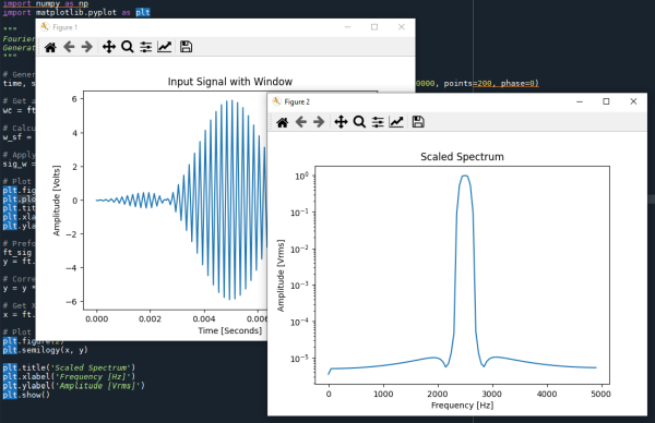
示例2 – 首先对输入数据应用窗口，欺骗FT认为波形不连续不存在

import FourierTransformHelperLib as ft
import matplotlib.pyplot as plt

"""
FourierTransformHelperLib - Article Example 2
Generate a signal, window it, and produce a properly scaled spectrum magnitude output
"""

# Generate a 5001 Hz Test Signal Tone with a 1.0 VRMS Amplitude
time, sig = ft.tone_sampling_points(amplitude=1.0, frequency=5001, 
                                    sampling_frequency=20000, points=200, phase=0)

# Get a window for the input data (Window)
wc = ft.window(window_type='fthp', points=len(sig))

# Calculate the sale factor of this generated window (Window)
w_sf = ft.window_scale_signal(window_coefficients=wc)

# Apply window to data (Window)
sig_w = sig * wc

# Plot input signal w/window
plt.figure(1)
plt.plot(time, sig_w)
plt.title('Input Signal with Window')
plt.xlabel('Time [Seconds]')
plt.ylabel('Amplitude [Volts]')

# Perform Fourier Transform and convert amplitude to magnitude
ft_sig = ft.ft_cpx(sig_w)
y = ft.complex_to_mag(ft_sig)

# Correct signal amplitude for window (Window)
y = y * w_sf

# Get X Scale for plotting
x = ft.frequency_bins(sampling_rate=10000, signal_length=len(sig))

# Plot Spectrum
plt.figure(2)
plt.semilogy(x, y)

plt.title('Scaled Spectrum')
plt.xlabel('Frequency [Hz]')
plt.ylabel('Amplitude [Vrms]')
plt.show()

如上所示，对输入数据应用窗口只需要另外4行代码（这些行在上面的代码中用(Window)注释）。将示例2的代码与示例1的代码进行比较。

示例3 – 带窗口和零填充的变换

import FourierTransformHelperLib as ft
import matplotlib.pyplot as plt

"""
FourierTransformHelperLib - Article Example 3
Generate a signal, window it, add zero padding to the FT,
and produce a properly scaled spectrum magnitude output
"""

# Generate a 5001 Hz Test Signal Tone with a 1.0 VRMS Amplitude
time, sig = ft.tone_sampling_points(amplitude=1.0, frequency=5001, 
                                    sampling_frequency=20000, points=200, phase=0)

# Get a window for the input data
wc = ft.window(window_type='fthp', points=len(sig))

# Calculate the sale factor of this generated window
w_sf = ft.window_scale_signal(window_coefficients=wc)

# Apply window to data
sig_w = sig * wc

# Plot input signal w/window
plt.figure(1)
plt.plot(time, sig_w)
plt.title('Input Signal with Window')
plt.xlabel('Time [Seconds]')
plt.ylabel('Amplitude [Volts]')

# Perform Fourier Transform and convert amplitude to magnitude
# Add the desired zero padding here (Padding)
ft_sig = ft.ft_cpx(sig_w, zero_padding=2000)
y = ft.complex_to_mag(ft_sig)

# Correct signal amplitude for window
y = y * w_sf

# Get X Scale (Remember that you added zero padding, so the length will be longer)
# (Padding)
x = ft.frequency_bins(sampling_rate=10000, signal_length=len(sig), 
                      zero_padding_length=2000)

# Plot Spectrum
plt.figure(2)
plt.semilogy(x, y)

plt.title('Scaled Spectrum')
plt.xlabel('Frequency [Hz]')
plt.ylabel('Amplitude [Vrms]')
plt.show()

在上面的示例3代码中，为示例2的代码添加零填充只需要修改两行，在上面的代码注释中标记为：(Padding)

FTHL基本使用步骤回顾

FTHL的设计在使用上是一致的。此外，信号和噪声信号也可以按照下面概述的基本步骤进行分析。

基本使用步骤 - 信号幅度分析

1. 计算信号的窗口系数和窗口比例因子。
2. 获取或生成输入数据。
3. 将窗口应用于输入数据。
4. 对窗口化输入数据执行FT。
5. 转换为幅度格式。
6. 应用窗口比例因子到数据。

结果：正确缩放的信号频谱

基本使用步骤 - 噪声信号分析

1. 计算信号的窗口系数和窗口比例因子。
2. 获取或生成输入数据。
3. 将窗口应用于输入数据。
4. 对窗口化输入数据执行FT。
5. 转换为幅度平方格式。
6. 如果需要：逐Bin平均幅度平方数据，然后对所有平均值重复步骤2-6。
7. 转换为幅度格式。
8. 应用窗口比例因子到数据。

结果：正确缩放的噪声信号频谱。

注意：信号和噪声必须区别对待的原因在参考文献[3]和[4]中有概述。

测试应用和示例描述

代码下载包含FTHL Python文件，以及八个示例测试脚本或手册，展示了如何执行各种常见的变换用例。这些手册示例应有助于根据您的具体需求运行FTHL。

下载中提供的示例代码手册

示例1 – 一个基本的DFT示例，生成数据并产生频谱输出
示例2 – 同上，但对测试数据应用了窗口
示例3 – 同上，但增加了零填充
示例4 – 同上，但使用最终的dBV[4]缩放进行显示
示例5 – 解释生成和平均噪声的正确方法
示例6 – 添加了噪声底的信号，以模拟真实信号
示例7 – 演示如何从FT输出中提取相位信息
示例8 – 演示如何对复杂的IQ输入数据执行完整的FT

完整库文档

下面提供了FTHL的每个部分和函数的完整库描述。该库还实现了Python Doc String注释，可在大多数Python IDE中提供“实时”帮助。

基本傅里叶变换核心函数

将实数或复数输入数据数组转换为正确缩放并切片的复数输出。参数zero_padding是可选的，如果包含，则会将该数量的零附加到输入数据长度。注意：FT必须知道添加的零的数量才能对结果进行正确的缩放。

def ft_cpx(signal, zero_padding=0):
    """
    Performs Fourier Transform on the input signal.
    Input may be real or complex.
    Input may be any length (not just powers of two).
    Uses SciPy.FFT as the base FFT implementation.

    Args:
        signal (float or Complex array): Input Signal to transform.
        zero_padding (int, optional): Additional zeros to pad the signal with
        Defaults to 0.

    Returns:
        complex: Resulting Fourier Transform as complex numbers.
        sliced to real frequencies only.
    """

频率跨度计算

此函数接收信号长度（加上您添加到FT的任何零填充），并计算上面FT函数返回的每个点的频率数组。这对于制作图的x轴很有用。

def frequency_bins(sampling_rate, signal_length, zero_padding_length=0):
    """
    Calculates the frequency of each Fourier Transform bin.
    Useful for plotting x axis of a Fourier Transform.

    Args:
        sampling_rate (float): Sampling Frequency in Hz
        signal_length (int): Length of input signal
        zero_padding_length (int, optional): Zero padding length. Defaults to 0.

    Returns:
        float array: Array of frequencies for each of the Fourier Transform Bins.
    """

傅里叶变换格式转换

这组函数将复数FT输出的复数或实数数据数组转换为更方便的最终用户格式。下载中包含的示例手册展示了这些格式转换的大部分内容及其用法。有几种输出格式可用

def complex_to_mag(cpx_arry):
    """Convert Complex Array to Magnitude Format Array.

    Args:
        cpx_arry (complex array): Complex Input Array.

    Returns:
        float array: Magnitude Format Output.
    """

def complex_to_mag2(cpx_arry):
    """Convert Complex Array to Magnitude Squared Format Array.

    Args:
        cpx_arry (complex array): Complex Input Array.

    Returns:
        float array: Magnitude Squared Format Output.
    """

def complex_to_dBV(cpx_arry):
    """Convert Complex Array to dBV Format Array.

    Args:
        cpx_arry (complex array): Complex Input Array.

    Returns:
        float array: dBV Format Output.
    """

def mag_to_mag2(mag_arry):
    """Convert Float Array to Magnitude Squared Format Array.

    Args:
        mag_arry (float array): Float Input Array.

    Returns:
        float array: Magnitude Squared Format Output.
    """

def mag_to_dBV(mag_arry):
    """Convert Float Array to dBV Format Array.

    Args:
        mag_arry (float array): Magnitude Input Array.

    Returns:
        float array: dBV Format Output.
    """

def mag2_to_mag(mag2_arry):
    """Convert Magnitude Squared Float Array to Magnitude Format Array.

    Args:
        mag2_arry (float array): Magnitude Squared Input Array.

    Returns:
        float array: Magnitude Format Output.
    """

def mag2_to_dBV(mag2_arry):
    """Convert Magnitude Squared Float Array to dBV Format Array.

    Args:
        mag2_arry (float array): Magnitude Squared Input Array.

    Returns:
        float array: dBV Format Output.
    """

def complex_to_phase_degrees(cpx_arry):
    """Convert Complex Number Input To Equivalent Phase Array In Degrees

    Args:
        cpx_arry (complex array): Input Array Of Complex Numbers.

    Returns:
        float array: Resulting Phase Angle In Degrees of Each Input Point
    """

def complex_to_phase_radians(cpx_arry):
    """Convert Complex Number Input To Equivalent Phase Array In Radians

    Args:
        cpx_arry (complex array): Input Array Of Complex Numbers.

    Returns:
        float array: Resulting Phase Angle In Radians of Each Input Point
    """

注意：计算出的相位在+/-PI间隔处总是有不连续性。为防止此问题，可以使用numpy.unwrap()函数尝试展开输入相位数组以消除跳跃式不连续性。这对于干净的信号效果很好，但随着信噪比的下降，从噪声中确定真正的不连续性变得更加困难。numpy.unwrap()函数是一个很好的起点，但对于真实世界的信号和低信噪比，当使用足够的信号平均时（请参阅上面下载中的示例5），性能最佳。

窗口系数生成

窗口用所需窗口名称的string值指定。该字符串与所需的点数一起传递到Coefficients函数。结果是一个双精度数组，可以通过与输入数据相乘来应用，还可以用于缩放因子例程之一，以确定窗口的增益或损失。窗口名称和参数在下面的附录A中指定，并在上面下载包中的文本文件列表中提供。

注意：此处生成的窗口长度不要添加任何零填充。

def window(window_type, points):
    """
    Generates the window coefficients for the specified window type.

    Parameters
    ----------
    window_type : string
        One of the following types of window may be specified,
    points : int
        Number of points total to generate.

    Returns
    -------
    numpy array of the generated window coefficients.
    Returns empty list if error.

    """

窗口分析和缩放

给定任何一组窗口系数，这些例程将确定所提供窗口数据数组的增益或损失。窗口系数可以是任何窗口，不限于FTHL提供的窗口。

window_scale_noise函数还考虑了Hz中的Bin宽度，以校正多个或分数赫兹的Bin宽度。有关如何使用此功能的更多信息，请参阅下载包中的示例5。

函数noise_bandwidth计算所提供窗口系数在Bin中的归一化等效噪声带宽[3]。

def window_scale_signal(window_coefficients):
    """
    Calculate Signal scale factor from window coefficient array.
    Designed to be applied to the "Magnitude" result.

    Args:
        window_coefficients (float array): window coefficients array

    Returns:
        float: Window scale correction factor for 'signal'
    """

def window_scale_noise(window_coefficients, sampling_frequency):
    """
    Calculate Noise scale factor from window coefficient array.
    Takes into account the bin width in Hz for the final result also.
    Designed to be applied to the "Magnitude" result.

    Args:
        window_coefficients (float array): window coefficients array
        sampling_frequency (_type_): sampling frequency in Hz

    Returns:
        float: Window scale correction factor for 'signal'
    """

def noise_bandwidth(window_coefficients):
    """
    Calculate Normalized, Equivalent Noise BandWidth from window coefficient array.

    Args:
        window_coefficients (float array): window coefficients array

    Returns:
        float: Equivalent Normalized Noise Bandwidth
    """  

信号生成

这些例程可用于生成测试信号进行模拟。

def tone_cycles(amplitude, cycles, points, phase):
    """
    Generates a sine wave tone, of a specified number of whole or partial cycles.

    Parameters
    ----------
    amplitude : float
        The desired amplitude in RMS volts.
    cycles : float
        The number of whole or partial sinewave cycles to generate.
    points : int
        Number of points total to generate.
    phase : float
        Phase angle in degrees to generate. The default is 0.0.

    Returns
    -------
    numpy array of the generated tone values.

    """

def tone_sampling_points(amplitude, frequency, sampling_frequency, points, phase):
    """
    Generates a sine wave tone, like it would be if sampled at a specified
    sampling frequency.

    Parameters
    ----------
    amplitude : float
        The desired amplitude in RMS volts.
    frequency : float
        Frequency in Hz of the generated tone.
    sampling_frequency : float
        Sampling frequency in Hz.
    points : int
        Number of points to generate.
    phase : float
        Phase angle in degrees to generate.

    Returns
    -------
    numpy tuple array of the time scale (x) and generated tone values (y).

    """

def tone_sampling_duration(amplitude, frequency, sampling_frequency, duration, phase):
    """
    Generates a sine wave tone, like it would be if sampled at a specified
    duration.

    Parameters
    ----------
    amplitude : float
        The desired amplitude in RMS volts.
    frequency : float
        Frequency in Hz of the generated tone.
    sampling_frequency : float
        Sampling frequency in Hz.
    duration : float
        Number of seconds to generate.
    phase : float
        Phase angle in degrees to generate.

    Returns
    -------
    numpy tuple array of the time scale (x) and generated tone values (y).

    """

噪声例程根据应用需求生成校准的噪声信号。可以指定功率谱密度（PSD）或使用伏特RMS值进行噪声。

功率谱密度（PSD）的单位是Vrms / rt-Hz（读作：每平方根赫兹伏特RMS）。

def noise_psd(amplitude_psd, sampling_frequency, points):
    """
    Generates a random noise stream of a given power spectral density
    in Vrms/rt-Hz. The noise is normally distributed, with a mean of 0.0 Volts.

    Parameters
    ----------
    density : float
        The desired noise density of the generated signal Vrms/rt-Hz.
    sampling_frequency : float
        Sampling frequency in Hz.
    number : int
        Number of points total to generate.

    Returns
    -------
    numpy array of the generated noise.

    """

def noise_rms(amplitude_rms, points):
    """
    Generates random noise stream of a given RMS voltage.
    The noise is normally distributed, with a mean of 0.0 Volts.

    Parameters
    ----------
    amplitude : float
        The desired amplitude in Volts RMS units..
    number : int
        Number of points total to generate.

    Returns
    -------
    numpy array of the generated noise.

    """

在您的项目中_使用“傅里叶变换助手库”_

从上面的链接下载FTHL_source_and_examples.zip。此zip文件包含FourierTransformHelperLib.py源文件，以及所有示例脚本。

最简单的用法是将FourierTransformHelperLib.py文件放在您的项目目录中，这样Python就能找到它。

将FourierTransformHelperLib.py源文件作为“import”添加到您的项目中，如下所示

import FourierTransformHelperLib as ft

系统要求

FourierTransformHelperLib.py使用python 3.9+和模块：numpy 1.22.2和scipy 1.8.0开发和测试。

参考文献

[1] Steve Hageman，“DSPLib - .NET 4的FFT / DFT傅里叶变换库”，
https://codeproject.org.cn/Articles/1107480/DSPLib-FFT-DFT-Fourier-Transform-Library-for-NET-6

[2] 帕塞瓦尔定理，
https://en.wikipedia.org/wiki/Parseval%27s_theorem

[3] G. Heinzel, A. Rudiger, and R. Schilling，“离散傅里叶变换（DFT）的频谱和功率谱密度估计，包括一个全面的窗口函数列表和一些新的平顶窗口。”，Max-Planck-Institut fur Gravitationsphysik，2002年2月15日

[4] Steve Hageman，“仪器仪表工程师实践者的傅里叶变换指南”，发表于EDN.com，2012年6月。
第一部分：理解DFT和FFT实现
第二部分：频谱泄漏和窗口化
第三部分：其他窗口类型、平均DFT及更多
精确测量小信号：实用指南

[5] dBV指的是以1伏特RMS为基准的20 *分贝（Decibels）的对数刻度。例如，
10 V RMS = 20 dBV
1 V RMS = 0 dBV
0.1 V RMS = - 20 dBV
另请参阅：https://en.wikipedia.org/wiki/Decibel

附录A – 包含的窗口类型

下面是FTHL中实现的窗口的性能参数表。

有关这些窗口的更多信息，请参阅参考文献[3]。
名称 峰值旁瓣电平 (dB) 平坦度 (dB) 3dB带宽 (bins) NENBW (bins)

名称	峰值旁瓣电平 (dB)	平坦度 (dB)	3dB带宽 (bins)	NENBW (bins)
矩形或无	13.3	3.9224	0.8845	1
Welch	21.3	2.2248	1.1535	1.2
Bartlett	26.5	1.8242	1.2736	1.3333
Hanning或Hann	31.5	1.4236	1.4382	1.5
Hamming	42.7	1.7514	1.3008	1.3628
Nuttall3	46.7	0.863	1.8496	1.9444
Nuttall4	60.9	0.6184	2.1884	2.31
Nuttall3A	64.2	1.0453	1.6828	1.7721
Nuttall3B	71.5	1.1352	1.6162	1.7037
Nuttall4A	82.6	0.7321	2.0123	2.1253
BH92	92	0.8256	1.8962	2.0044
Nuttall4B	93.3	0.8118	1.9122	2.0212

名称	峰值旁瓣电平 (dB)	平坦度 (dB)	3dB带宽 (bins)	NENBW (bins)
SFT3F	31.7	0.0082	3.1502	3.1681
SFT3M	44.2	0.0115	2.9183	2.9452
FTNI	44.4	0.0169	2.9355	2.9656
SFT4F	44.7	0.0041	3.7618	3.797
SFT5F	57.3	0.0025	4.291	4.3412
SFT4M	66.5	0.0067	3.3451	3.3868
FTHP	70.4	0.0096	3.3846	3.4279
HFT70	70.4	0.0065	3.372	3.4129
FTSRS	76.6	0.0156	3.7274	3.7702
SFT5M	89.9	0.0039	3.834	3.8852
HFT90D	90.2	0.0039	3.832	3.8832
HFT95	95	0.0044	3.759	3.8112
HFT116D	116.8	0.0028	4.1579	4.2186
HFT144D	144.1	0.0021	4.4697	4.5386
HFT169D	169.5	0.0017	4.7588	4.8347
HFT196D	196.2	0.0013	5.0308	5.1134
HFT223D	223	0.0011	5.3	5.3888
HFT248D	248.4	0.0009	5.5567	5.6512

HFT248D类型的窗口在FTHL中会调用为：‘hft248d’。

注意：表1和表2中列出的值来自参考文献[3]。

历史

• 版本1.0 - 2022年4月13日 - 首次发布